STATISTICS

Chapter -6

STATISTICS

Introduction
In fact, you went a step further by studying certain numerical representatives of the ungrouped data, also called measures of central tendency, namely, mean, median and mode. In this chapter, we shall extend the study of these three measures, i.e., mean, median and mode from ungrouped data to that of grouped data. We shall also discuss the concept of cumulative frequency, the cumulative frequency distribution and how to draw cumulative frequency curves, called ogives.

Mean of Grouped Data
The mean (or average) of observations, as we know, is the sum of the values of all the observations divided by the total number of observations. From Class IX, recall that if x₁, x₂,…., x_n are observations with respective frequencies f₁,  f₂, …., f_nx_n, then this means observation x₁ occurs f₁ times, x₂ occurs f₂ times, and so on.
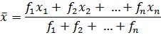
Now, the sum of the values of all the observations = f₁x₁ + f₂x₂ + … + f_nx_n, and the number of observations = f₁ + f₂ + … + f_n.
So, the mean    of the data is given by

Recall that we can write this in short form by using the Greek letter ∑ (capital sigma) which means summation. That is,
                      
Which, more briefly, is written as  if it is understood that I varies from 1 to n.
So, from Table 14.4, the mean of the deviations,
Now, let us find the relation between d and x.
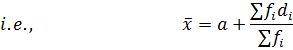
Since in obtaining d_i, we subtracted ‘a’ from each x_i, so, in order to get the mean  we need to add ‘a’ to . This can be explained mathematically as:

Mean of deviations,     

So,                               

Median of Grouped Data
As you have studied in Class IX, the median is a measure of central tendency which gives the value of the middle-most observation in the data. Recall that for finding the median of ungrouped data, we first arrange the data values of the observations in ascending order. Then, if n is odd, the median is the observation. And, if is even, then the

After finding the median class, we use the following formula for calculating the median.
         
Where                   l = lower limit of median class,
                                 n = Number of observations,
                                cf = Cumulative frequency of class preceding the median class,
                                f = Frequency of median class,
                              h = Class size (assuming class size to be equal).

Remarks:
1. There is an empirical relationship between the three measures of central tendency:
2 Median = Mode + 2 Mean
3. The median of grouped data with unequal class sizes can also be calculated. However, we shall not discuss it here. 

Mode of Grouped Data

Recall from Class IX, a mode is that value among the observations which occurs most often, that is, the value of the observation having the maximum frequency. Further, we discussed finding the mode of ungrouped data. Here, we shall discuss ways of obtaining a mode of grouped data. It is possible that more than one value may have the same maximum frequency. In such situations, the data is said to be multimodal.  Though grouped data can also be multimodal, we shall restrict ourselves to problems having a single mode only.
 
Where l = lower limit of the modal class,
h = size of the class interval (assuming all class sizes to be equal),
f₁ = frequency of the modal class,
f₀ = frequency of the class preceding the modal class,
f₂ = frequency of the class succeeding the modal class.
Let us consider the following examples to illustrate the use of this formula.

Graphical Representation of Cumulative Frequency Distribution
As we all know, pictures speak better than words. A graphical representation helps us in understanding given data at a glance. In Class IX, we have represented the data through bar graphs, histograms and frequency polygons. Let us now represent a cumulative frequency distribution graphically.
For example, let us consider the cumulative frequency distribution given in Table 14.13.
Recall that the values 10, 20, 30,. . ., 100 are the upper limits of the respective class intervals. To represent the data in the table graphically, we mark the upper limits of the class intervals on the horizontal axis (x-axis) and their corresponding cumulative frequencies on the vertical axis (y-axis), choosing a convenient scale. The scale may not be the same on both the axis. Let us now plot the points corresponding to the ordered pairs given by (upper limit, corresponding cumulative frequency), i.e., (10, 5), (20, 8), (30, 12), (40, 15), (50, 18), (60, 22), (70, 29), (80, 38), (90, 45), (100, 53) on a graph paper and join them by a free hand smooth curve. The curve we get is called a cumulative frequency curve, or an ogive (of the less than type).