Introduction

Chapter -14

Probability

Introduction

In Class IX, you have studied about experimental (or empirical) probabilities of events which were based on the results of actual experiments. We discussed an experiment of tossing a coin 1000 times in which the frequencies of the outcomes were as follows:
                             Head: 455                      Tails: 545
Based on this experiment, the empirical probability of a head is  that of getting a tail is 0.545. (Also see Example 1, Chapter 15 of Class IX Mathematics Textbook.) Note that these probabilities are based on the results of an actual experiment of tossing a coin 1000 times. For this reason, they are called experimental or empirical probabilities. In fact, experimental probabilities are based on the results of actual experiments and adequate recordings of the happening of the events. Moreover, these probabilities are only ‘estimates’. If we perform the same experiment for another 1000 times, we may get different data giving different probability estimates.
In Class IX, you tossed a coin many times and noted the number of times it turned up heads (or tails) (refer to Activities 1 and 2 of Chapter 15). You also noted that as the number of tosses of the coin increased, the experimental probability of getting a head (or tail) came closer and closer to the number  Not only you, but many other Persons from different parts of the world have done this kind of experiment and recorded the number of heads that turned up.
For example, the eighteenth century French naturalist Comte de Buffon tossed a coin 4040 times and got 2048 heads. The experimental probability of getting a head, in this case, was    i.e., 0.507. J.E. Kerrich, from Britain, recorded 5067 heads in 10000 tosses of a coin. The experimental probability of getting a head, in this case, was  Statistician Karl Pearson spent some more time, making 24000 tosses of a coin. He got 12012 heads, and thus, the experimental probability of a head obtained by him was 0.5005.
Now, suppose we ask, ‘What will the experimental probability of a head be if the experiment is carried on upto, say, one million times? Or 10 million times? And so on?’ You would intuitively feel that as the number of tosses increases, the experimental probability of a head (or a tail) seems to be settling down around the number 0.5 , i.e., 1/2,  which is what we call the theoretical probability of getting a head (or getting a tail), as you will see in the next section. In this chapter, we provide an introduction to the theoretical (also called classical) probability of an event, and discuss simple problems based on this concept.

Probability — A Theoretical Approach
Let us consider the following situation:

Suppose a coin is tossed at random.
We know, in advance, that the coin can only land in one of two possible ways — either head up or tail up (we dismiss the possibility of its ‘landing’ on its edge, which may be possible, for example, if it falls on sand). We can reasonably assume that each outcome, head or tail, is as likely to occur as the other. We refer to this by saying that the outcomes head and tail, are equally likely.
For another example of equally likely outcomes, suppose we throw a die once. For us, a die will always mean a fair die. What are the possible outcomes? They are 1, 2, 3, 4, 5, 6. Each number has the same possibility of showing up. So the equally likely outcomes of throwing a die are 1, 2, 3, 4, 5 and 6.
Are the outcomes of every experiment equally likely? Let us see.
Suppose that a bag contains 4 red balls and 1 blue ball, and you draw a ball without looking into the bag. What are the outcomes? Are the outcomes — a red ball and a blue ball equally likely? Since there are 4 red balls and only one blue ball, you would agree that you are more likely to get a red ball than a blue ball. So, the outcomes (a red ball or a blue ball) are not equally likely. However, the outcome of drawing a ball of any colour from the bag is equally likely. So, all experiments do not necessarily have equally likely outcomes.
However, in this chapter, from now on, we will assume that all the experiments have equally likely outcomes.
In Class IX, we defined the experimental or empirical probability P(E) of an event E as

The empirical interpretation of probability can be applied to every event associated with an experiment which can be repeated a large number of times. The requirement of repeating an experiment has some limitations, as it may be very expensive or unfeasible in many situations. Of course, it worked well in coin tossing or die throwing experiments. But how about repeating the experiment of launching a satellite in order to compute the empirical probability of its failure during launching, or the repetition of the phenomenon of an earthquake to compute the empirical probability of a multistoreyed building getting destroyed in an earthquake?
In experiments where we are prepared to make certain assumptions, the repetition of an experiment can be avoided, as the assumptions help in directly calculating the exact (theoretical) probability. The assumption of equally likely outcomes (which is valid in many experiments, as in the two examples above, of a coin and of a die) is one such assumption that leads us to the following definition of probability of an event.
The theoretical probability (also called classical probability) of an event E, written as P(E), is defined as

Where we assume that the outcomes of the experiment are equally likely.
We will briefly refer to theoretical probability as probability.
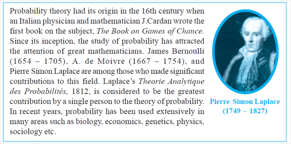
This definition of probability was given by Pierre Simon Laplace in 1795.

Let us find the probability for some of the events associated with experiments where the equally likely assumption holds.