 Kaysons Publication
NUMBER SYSTEMS
- Books Name
- Kaysons Academy Maths Foundation Book
- Publication
- Kaysons Publication
- Course
- JEE
- Subject
- Maths
Chapter -1
Number Systems
Introduction
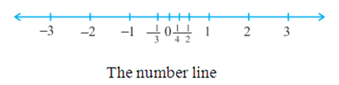
In your earlier classes, you have learnt about the number line and how to represent various types of numbers on it.
Just imagine you start from zero and go on walking along this number line in the positive direction. As far as your eyes can see, there are numbers, numbers and numbers!
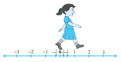
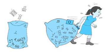
Now suppose you start walking along the number line, and collecting some of the numbers. Get a bag ready to store them!
You might begin with picking up only natural numbers like 1, 2, 3, and so on. You know that this list goes on forever. (Why is this true?) So, now your bag contains infinitely many natural numbers! Recall that we denote this collection by the symbol N.
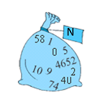
Now turn and walk all the way back, pick up zero and put it into the bag. You now have the collection of whole numbers which is denoted by the symbol W.

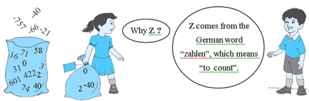
Now, stretching in front of you are many, many negative integers. Put all the negative integers into your bag. What is your new collection? Recall that it is the collection of all integers, and it is denoted by the symbol Z.
Are there some numbers still left on the line? Of course! There are numbers like
![]()
Collection of rational numbers. The collection of rational numbers is denoted by Q.
‘Rational’ comes from the word ‘ratio’, and Q comes from the word ‘quotient’.
You may recall the definition of rational numbers:
A number ‘r’ is called a rational number, if it can be written in the form P/q, where p and q are integers and q ≠ 0. (Why do we insist that q ≠ 0?)
Notice that all the numbers now in the bag can be written in the form , where p and q are integers and q ≠ 0. For example, – 25 can be written as (-25)/1; here p = – 25 and q = 1. Therefore, the rational numbers do not have a unique representation in the form p/q, where p and q are integers and q ≠ 0. For example, 1/2=2/4=10/20=25/50=47/94, and so on. These are equivalent rational numbers (or fractions). However,
When we say that p/q is a rational number, or when we represent p/q on the number line, we assume that q ≠ 0 and that p and q have no common factors other than 1 (that is, p and q are co-prime). So, on the number line, among the infinitely many fractions equivalent to 1/2, we will choose 1/2 to represent all of them.
Now, let us solve some examples about the different types of numbers, which you have studied in earlier classes.
Irrational Numbers
We saw, in the previous section, that there may be numbers on the number line that are not rationals. In this section, we are going to investigate these numbers. So far, all The numbers you have come across, are of the form p/q, where p and q are integers and q ≠ 0. So, you may ask: are there numbers which are not of this form? There are indeed such numbers. Let us formally define these numbers.
A number’s’ is called irrational, if it cannot be written in the form p/q, where p and q are integers and q ≠ 0. we call the collection of real numbers,
Which is denoted by R.? Therefore, a real number is either rational or irrational. So, we can say that every real number is represented by a unique point on the number line. Also, every point on the number line represents a unique real number. This is why we call the number line, the real number line.
Let us see how we can locate some of the irrational numbers on the number line.
We have just seen that OB = √2. Using a compass with centre O and radius OB, draw an arc intersecting the number line at the point P. Then P corresponds to √2 on the number line.
The decimal expansion of a rational number is terminating or non- terminating recurring. Moreover, a number whose decimal expansion is terminating or non-terminating recurring is rational.
The decimal expansion of an irrational number is non-terminating non-recurring. Moreover, a number whose decimal expansion is non-terminating non-recurring is irrational.
Representing Real Numbers on the Number Line
Suppose we want to locate 2.665 on the number line. We know that this lies between 2and 3.So, let us look closely at the portion of the number line between 2 and 3. Suppose we divide this into 10 equal parts and mark each point of division as (i). Then the first mark to the right of 2 will represent 2.1, the second 2.2, and so on. You might be finding some difficulty in observing these points of division between 2 and 3
(i). To have a clear view of the same, you may take a magnifying glass and look at the portion between 2 and 3. It will look like what you see
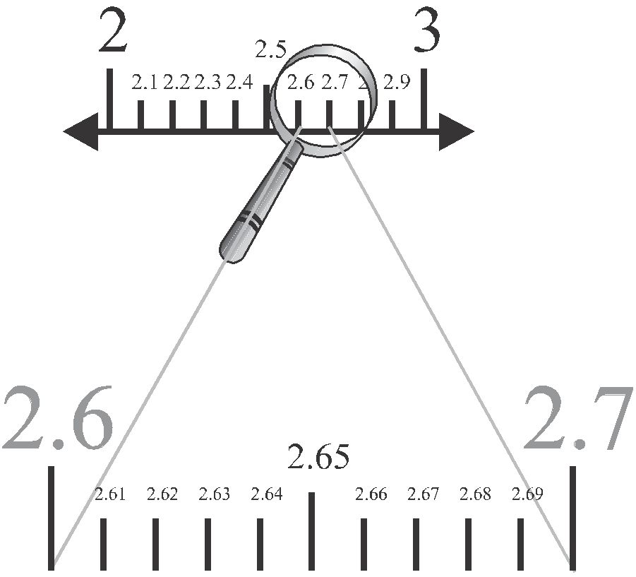
(ii). Now, 2.665 lie between 2.6 and 2.7. So, let us focus on the portion between 2.6 and 2.7. We imagine dividing this again into ten equal parts. The first mark will represent 2.61, the next 2.62, and so on. To see this clearly, we magnify this as shown (ii).
Operations on Real Numbers
- Books Name
- Kaysons Academy Maths Foundation Book
- Publication
- Kaysons Publication
- Course
- JEE
- Subject
- Maths
Operations on Real Numbers
You have learnt, in earlier classes that rational numbers satisfy the commutative, associative and distributive laws for addition and multiplication. Moreover, if we add, subtract, multiply or divide (except by zero) two rational numbers, we still get a rational number (that is, rational numbers are ‘closed’ with respect to addition, subtraction, multiplication and division). It turns out that irrational numbers also satisfy the commutative, associative and distributive laws for addition and multiplication. However, the sum, difference, quotients and products of irrational numbers are not always

Let us look at what happens when we add and multiply a rational number with an irrational number. For example, ![]() is irrational. What about 2 +
is irrational. What about 2 + ![]() and
and ![]() since
since ![]() has a non-recurring decimal expansion, the same is true for 2 +
has a non-recurring decimal expansion, the same is true for 2 + ![]() and
and![]() . Therefore, both 2 +
. Therefore, both 2 + ![]() and
and ![]() are also irrational numbers.
are also irrational numbers.
Introduction
- Books Name
- Kaysons Academy Maths Foundation Book
- Publication
- Kaysons Publication
- Course
- JEE
- Subject
- Maths
Chapter -2
Polynomials
Introduction
In this chapter, we shall start our study with a particular type of algebraic expression, called polynomial, and the terminology related to it. We shall also study the Remainder Theorem and Factor Theorem and their use in the factorisation of polynomials. In addition to the above, we shall study some more algebraic identities and their use in factorisation and in evaluating some given expressions.
Polynomials in One Variable
Let us begin by recalling that a variable is denoted by a symbol that can take any real value. We use the letters x, y, z, etc. to denote variables. Notice that 2x, 3x, – x, ![]() are algebraic expressions. All these expressions are of the form (a constant) × x. Now suppose we want to write an expression which is (a constant) × (a variable) and we do not know what the constant is. In such case, we write the constant as a, b, c, etc. So the expression will be ax, say.
are algebraic expressions. All these expressions are of the form (a constant) × x. Now suppose we want to write an expression which is (a constant) × (a variable) and we do not know what the constant is. In such case, we write the constant as a, b, c, etc. So the expression will be ax, say.
However, there is a difference between a letter denoting a constant and a letter denoting a variable. The values of the constants remain the same throughout a particular situation, that is, the values of the constants do not change in a given problem, but the value of a variable can keep changing.
Now, consider a square of side 3 units What is its perimeter? You know that the perimeter of a square is the sum of the lengths of its four sides. Here, each side is 3 units. So, its perimeter is 4 × 3, i.e., 12 units. What will be the perimeter if each side of the square is 10 units? The perimeter is 4 × 10, i.e., 40 units. In case the length of each side is x units, the perimeter is given by 4x units. So, as the length of the side varies, the perimeter varies.
Expressions of this form are called polynomials in one variable. In the examples above, the variable is x. For instance, x3 – x2 + 4x + 7is a polynomial in x. For instance, x3 – x2 + 4x + 7 is a polynomial in x. Similarly, 3y2 + 5y is a polynomial in the variable y and t2 + 4 is a polynomial in the variable t.
In the polynomial x2 + 2x, the expressions x2 and 2x are called the terms of the polynomial. Similarly, the polynomial 3y2 + 5y + 7 has there terms, namely, 3y2, 5y and 7. Can you write the terms of the polynomial –x3 + 4x2 + 7x – 2 ? This polynomial has 4 terms, namely, –x3, 4x2, 7x and –2.
Each term of a polynomial has a coefficient. So, in –x3 + 4x2 + 7x – 2, the coefficient of x3 is –1, the coefficient of x2 is 4, the coefficient of x is 7 and –2 is the coefficient of xo (Remember, xo = 1). Do you know the coefficient of x in x2 – x + 7? It is –1.
2 is also a polynomial. In fact, 2, –5, 7 etc. are example of constant polynomials. The constant polynomial 0 is called the zero polynomial. This plays a very important role in the collection of all polynomials, as you will see in the higher classes.
Now, look at the polynomial p(x) = 3x7 – 4x6 + x + 9. What is the term with the highest power of x ? It is 3x7. The exponent of x in this term is 7. Similarly, in the polynomial q(y) = 5y6 – 4y2 – 6, the term with the highest power of y is 5y6 and the exponent of y in this term is 6. We call the highest power of the variable in a polynomial as the degree of the polynomial. So, the degree of the polynomial 3x7 – 4 x6 + x + 9 is 7 and the degree of the polynomial 5y6 – 4y2 – 6 is 6. The degree of a non-zero constant polynomial is zero.
Now, that you have seen what a polynomial of degree 1, degree 2, or degree 3 looks like, can you write down a polynomial in one variable of degree n for any natural number n? A polynomial in one variable x of degree n is an expression of the form
anxn + an – 1xx – 1 + … + a1x + ao
Where ao, a1, a2, …, an are constants and an ≠ 0.
In particular, if ao = a1 = a2 = a3 = … = an = 0 (all the constants are zero), we get the zero polynomial, which is denoted by 0. What is the degree of the zero polynomial? The degree of the zero polynomial is not defined.
Remainder Theorem
- Books Name
- Kaysons Academy Maths Foundation Book
- Publication
- Kaysons Publication
- Course
- JEE
- Subject
- Maths
Remainder Theorem
Let us consider two numbers 15 and 6. You know that when we divide 15 by 6, we get the quotient 2 and remainder 3. Do you remember how this fact is expressed? We write 15 as
15 = (6 × 2) + 3
We observe that the remainder 3 is less than the divisor 6. Similarly, if we divide12 by 6, we get
12 = (6 × 2) + 0
What is the remainder here? Here the remainder is 0, and we say that 6 is a factor of 12 or 12 is a multiple of 6.
Now, the question is: can we divide one polynomial by another? To start with, let us try and do this when the divisor is a monomial. So, let us divide the polynomial 2x3 + x2 + x by the monomial x.
We have (2x3 + x2 + x) ÷ x = ![]()
= 2x2 + x + 1
In fact, you may have noticed that x is common to each term of 2x3 + x2 + x. So we can write
(2x3 + x2 + x as x(2x2 + x + 1).
We say that x and 2x2 + x + 1 are factors of 2x3 + x2 + x, and 2x3 + x2 + x is a multiple of x as well as a multiple of 2x2 + x + 1.
Consider another pair of polynomials 3x2 + x + 1 and x.
Here, (3x2 + x + 1) ÷ x = (3x2 ÷ x) + (x ÷ x) + (1 + x).
We see that we cannot divide 1 by x to get a polynomial term. So in this case we stop here, and note that 1 is the remainder. Therefore, we have
3x2 + x + 1 = {x × (3x + 1) } + 1
In this case, 3x + 1 is the quotient and 1 is the remainder. Do you think that x is a factor of 3x2 + x + 1? Since the remainder is not zero, it is not a factor.
Now let us consider an example to see how we can divide a polynomial by any non-zero polynomial.
i.e., Dividend = (Divisor × Quotient) + Remainder
In general, if p(x) and g(x) are two polynomials such that degree of p(x) ≥ degree of g(x) and g(x) ≠ 0, then we can find polynomials q(x) and r(x) such that:
p(x) = g(x)q(x) + r(x),
Where r (x) = 0 or degree of r(x) < degree of g(x). Here we say that p(x) divided by g(x), gives q(x) as quotient and r(x) as remainder.
In the example above, the divisor was a linear polynomial. In such a situation, let us see if there is any link between the remainder and certain values of the dividend.
Remainder Theorem: Let p(x ) be any polynomial of degree greater than or equal to one and let a be any real number. If p (x) is divided by the linear polynomial x – a, then the remainder is p (a).
Proof: Let p(x) be any polynomial with degree greater than or equal to 1. Suppose that when p(x) is divided by x – a, the quotient is q(x) and the remainder is r (x), i.e.,
p(x) = (x – a) q(x) + r (x)
Since the degree of x – a is 1 and the degree of r(x) is less than the degree of x – a, the degree of r(x) = 0. This means that r(x) is a constant, say r.
So, for every value of x, r(x) = r.
Therefore, p(x) = (x – a) q(x) + r
In particular, if x = a, this equation gives us
p(a) = (a – a) q(a) + r = r,
Which proves the theorem?
Let us use this result in another example.
Factorization of Polynomials
- Books Name
- Kaysons Academy Maths Foundation Book
- Publication
- Kaysons Publication
- Course
- JEE
- Subject
- Maths
Factorization of Polynomials
Let us now look at the situation of Example 10 above more closely. It tells us that since the remainder, ![]() (2t + 1) is a factor of q(t), i.e., q(t) = (2t + 1) g(t) for some polynomial g(t). This is a particular case of the following theorem.
(2t + 1) is a factor of q(t), i.e., q(t) = (2t + 1) g(t) for some polynomial g(t). This is a particular case of the following theorem.
Factor Theorem: If p(x) is a polynomial of degree n > 1 and a is any real number, then (i)
x – a is a factor of p(x), if p(a) = 0, and (ii) p(a) = 0, if x – a is a factor of p(x).
Proof: By the Remainder Theorem, p(x)=(x – a) q(x) + p(a).
(i) If p(a) = 0, then p(x) = (x – a) q(x), which shows that x – a is a factor of p(x).
(ii) Since x – a is a factor of p(x), p(x) = (x – a) g(x) for same polynomial g(x). In this case,
p(a) = (a – a) g(a) = 0.
Algebraic Identities
- Books Name
- Kaysons Academy Maths Foundation Book
- Publication
- Kaysons Publication
- Course
- JEE
- Subject
- Maths
Algebraic Identities
From your earlier classes, you may recall that an algebraic identity is an algebraic equation that is true for all values of the variables occurring in it. You have studied the following algebraic identities in earlier classes:
Identity I: (x + y)2 = x2 + 2xy + y2
Identity II: (x – y)2 = x2 – 2xy + y2
Identity III: x2 – y2 = (x + y) (x – y)
Identity IV: (x + a) (x + b) = x2 + (a + b)x + ab
You must have also used some of these algebraic identities to factorise the algebraic expressions. You can also see their utility in computations.
Introduction
- Books Name
- Kaysons Academy Maths Foundation Book
- Publication
- Kaysons Publication
- Course
- JEE
- Subject
- Maths
Chapter -3
Coordinate Geometry
Introduction
You have already studied how to locate a point on a number line. You also know how to describe the position of a point on the line. There are many other situations, in which to find a point we are required to describe its position with reference to more than one line. For example, consider the following situations:
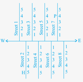
In Fig., there is a main road running in the East-West direction and streets with numbering from West to East. Also, on each street, house numbers are marked. To look for a friend’s house here, is it enough to know only one reference point? For instance, if we only know that she lives on Street 2, will we be able to find her house easily? Not as easily as when we know two pieces of information about it, namely, the number of the street on which it is situated, and the house number. If we want to reach the house which is situated in the 2nd street and has the number 5, first of all we would identify the 2nd street and then the house numbered 5 on it. In Fig., H shows the location of the house. Similarly, P shows the location of the house corresponding to Street number 7 and House number 4.
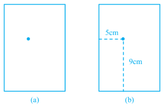
Suppose you put a dot on a sheet of paper [Fig. (a)]. If we ask you to tell us the position of the dot on the paper, how will you do this? Perhaps you will try in some such manner: “The dot is in the upper half of the paper”, or “It is near the left edge of the paper”, or “It is very near the left hand upper corner of the sheet”. Do any of these statements fix the position of the dot precisely? No! But, if you say “The dot is nearly 5 cm away from the left edge of the paper”, it helps to give some idea but still does not fix the position of the dot. A little thought might enable you to say that the dot is also at a distance of 9 cm above the bottom line. We now know exactly where the dot is!
For this purpose, we fixed the position of the dot by specifying its distances from two fixed lines, the left edge of the paper and the bottom line of the paper [Fig. (b)]. In other words, we need two independent information’s for finding the position of the dot.
Now, perform the following classroom activity known as ‘Seating Plan’.
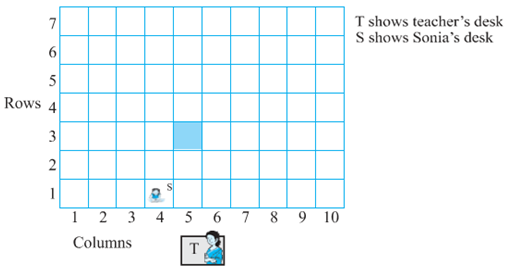
Activity 1 (Seating Plan): Draw a plan of the seating in your classroom, pushing all the desks together. Represent each desk by a square. In each square, write the name of the student occupying the desk, which the square represents. Position of each student in the classroom is described precisely by using two independent informations:
(i) The column in which she or he sits,
(ii) The row in which she or he sits.
If you are sitting on the desk lying in the 5th column and 3rd row (represented by the shaded square in Fig. your position could be written as (5, 3), first writing the column number, and then the row number. Is this the same as (3, 5)? Write down the names and positions of other students in your class. For example, if Sonia is sitting in the 4th column and 1st row, write S(4,1). The teacher’s desk is not part of your seating plan. We are treating the teacher just as an observer.
Cartesian System
- Books Name
- Kaysons Academy Maths Foundation Book
- Publication
- Kaysons Publication
- Course
- JEE
- Subject
- Maths
Cartesian System
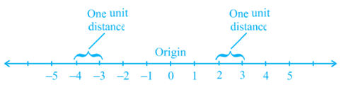
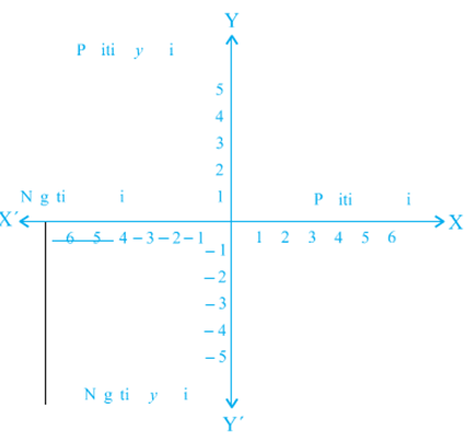
You have studied the number line in the chapter on ‘Number System’. On the number line, distances from a fixed point are marked in equal units positively in one direction and negatively in the other. The point from which the distances are marked is called the origin. We use the number line to represent the numbers by marking points on a line at equal distances. If one unit distance represents the number ‘1’, then 3 units distance represents the number ‘3’, ‘0’ being at the origin. The point in the positive direction at a distance r from the origin represents the number r. The point in the negative direction at a distance r from the origin represents the number −r. Locations of different numbers on the number line are shown in Fig.
Descartes invented the idea of placing two such lines perpendicular to each other on a plane, and locating points on the plane by referring them to these lines. The perpendicular lines may be in any direction such as in Fig. But, when we choose
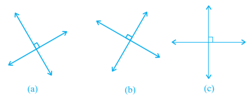
these two lines to locate a point in a plane in this chapter, one line will be horizontal and the other will be vertical, as in Fig.(c).
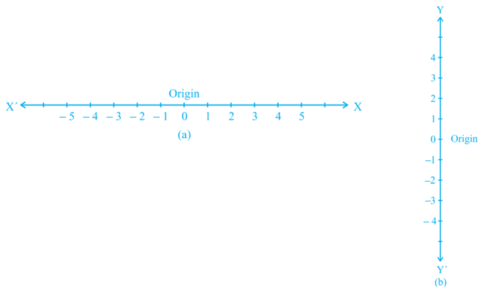
These lines are actually obtained as follows: Take two number lines, calling them X′X and Y′Y. Place X′X horizontal [as in Fig.(a)] and write the numbers on it just as written on the number line. We do the same thing with Y′Y except that Y′Y is vertical, not horizontal [Fig.(b)].
Combine both the lines in such a way that the two lines cross each other at their zeroes, or origins (Fig. 3.8). The horizontal line X′X is called the x - axis and the vertical line Y′Y is called the y - axis. The point where X′X and Y′Y cross is called the origin, and is denoted by O. Since the positive numbers lie on the directions OX and OY, OX and OY are called the positive directions of the x - axis and the y - axis, respectively. Similarly, OX′ and OY′ are called the negative directions of the x - axis and the y - axis, respectively.
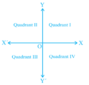
You observe that the axes (plural of the word ‘axis’) divide the plane into four parts. These four parts are called the quadrants (one fourth part), numbered I, II, III and IV anticlockwise from OX (see Fig.3.9). So, the plane consists of the axes and these quadrants. We call the plane, the Cartesian plane, or the coor donate plane, or the xy-plane. The axes are called the coordinate axes.
Now, let us see why this system is so basic to mathematics, and how it is useful. Consider the following diagram where the axes are drawn on graph paper. Let us see the distances of the points P and Q from the axes. For this, we draw perpendiculars PM on the x - axis and PN on the y - axis. Similarly, we draw perpendiculars QR and QS as shown in Fig. 3.10.
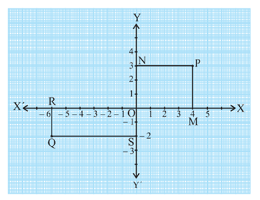
You find that
(i) The perpendicular distance of the point P from the y - axis measured along the positive direction of the x - axis is PN = OM = 4 units.
(ii) The perpendicular distance of the point P from the x - axis measured along the positive direction of the y - axis is PM = ON = 3 units.
(iii) The perpendicular distance of the point Q from the y - axis measured along the negative direction of the x - axis is OR = SQ = 6 units.
(iv) The perpendicular distance of the point Q from the x - axis measured along the negative direction of the y - axis is OS = RQ = 2 units.
Now, using these distances, how can we describe the points so that there is no confusion?
We write the coordinates of a point, using the following conventions:
(i) The x - coor dinate of a point is its perpendicular distance from the y - axis measured along the x -axis (positive along the positive direction of the x - axis and negative along the negative direction of the x - axis). For the point P, it is
+ 4 and for Q, it is – 6. The x - coordinate is also called the abscissa.
(ii) The y - coor dinate of a point is its perpendicular distance from the x - axis measured along the y - axis (positive along the positive direction of the y - axis and negative along the negative direction of the y - axis). For the point P, it is
+ 3 and for Q, it is –2. The y - coordinate is also called the ordinate.
(iii) In stating the coordinates of a point in the coordinate plane, the x - coordinate comes first, and then the y - coordinate. We place the coordinates in brackets.
Hence, the coordinates of P are (4, 3) and the coordinates of Q are (– 6, – 2). Note that the coordinates describe a point in the plane uniquely. (3, 4) is not the same as (4, 3).
Surface Area of a Cuboid and a Cube
- Books Name
- Kaysons Academy Maths Foundation Book
- Publication
- Kaysons Publication
- Course
- JEE
- Subject
- Maths
Chapter -11
SURFACE AREAS AND VOLUMES
Surface Area of a Cuboid and a Cube
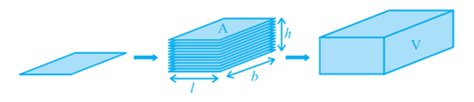
Have you looked at a bundle of many sheets of paper? How does it look? Does it look like what you see in Fig.
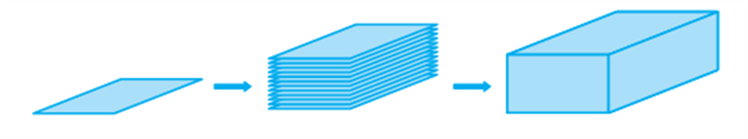
That makes up a cuboid. How much of brown paper would you need, if you want to cover this cuboid? Let us see:
First we would need a rectangular piece to cover the bottom of the bundle. That would be as shown in Fig (a)

Then we would need two long rectangular pieces to cover the two side ends. Now, it would look like Fig (b).
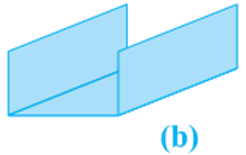
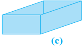
Now to cover the front and back ends, we would need two more rectangular pieces of a different size. With them, we would now have a figure as shown in Fig (c).
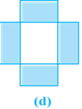
This figure, when opened out, would look like Fig (d).
Finally, to cover the top of the bundle, we would require another rectangular piece exactly like the one at the bottom, which if we attach on the right side, it would look like Fig (e).
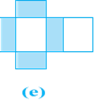
So we have used six rectangular pieces to cover the complete outer surface of the cuboid.
This shows us that the outer surface of a cuboid is made up of six rectangles (in fact, rectangular regions, called the faces of the cuboid), who’s areas can be found by multiplying length by breadth for each of them separately and then adding the six areas together.
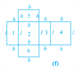
Now, if we take the length of the cuboid as l, breadth as b and the height as h, then the figure with these dimensions would be like the shape you see in Fig (f).
So, the sum of the areas of the six rectangles is:
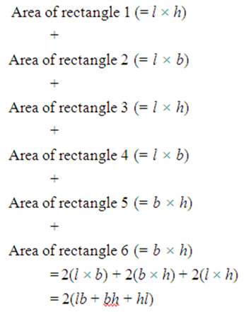
This gives us:
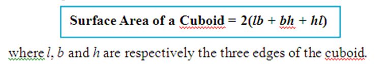
Where l, b and h are respectively the three edges of the cuboid.
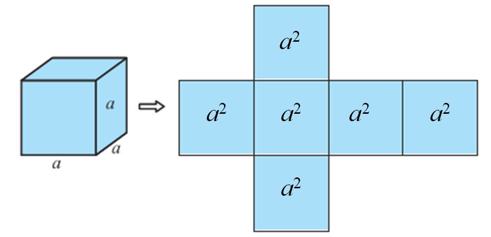
Recall that a cuboid, whose length, breadth and height are all equal, is called a cube. If each edge of the cube is a, then the surface area of this cube would be
![]()
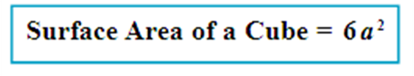
Where a is the edge of the cube.
Suppose, out of the six faces of a cuboid, we only find the area of the four faces, leaving the bottom and top faces. In such a case, the area of these four faces is called the lateral surface area of the cuboid. So, lateral surface area of a cuboid of length l, breadth b and height h is equal to 2lh + 2bh or 2(l + b)h. Similarly, lateral surface area of a cube of side a is equal to 4a2.
Keeping in view of the above, the surface area of a cuboid (or a cube) is sometimes also referred to as the total surface area.
Surface Area of a Right Circular Cylinder
- Books Name
- Kaysons Academy Maths Foundation Book
- Publication
- Kaysons Publication
- Course
- JEE
- Subject
- Maths
Surface Area of a Right Circular Cylinder
If we take a number of circular sheets of paper and stack them up as we stacked up rectangular sheets earlier, what would we get (see Fig.)
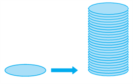
Here, if the stack is kept vertically up, we get what is called a right circular cylinder, since it has been kept at right angles to the base, and the base is circular. Let us see what kind of cylinder is not a right circular cylinder.
In Fig (a), you see a cylinder, which is certainly circular, but it is not at right angles to the base. So, we can not say this a right circular cylinder.
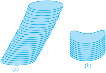
Of course, if we have a cylinder with a non circular base, as you see in Fig (b). then we also cannot call it a right circular cylinder.
So curved surface area of the cylinder = area of the rectangular sheet = length × breadth
= perimeter of the base of the cylinder x h ![]()
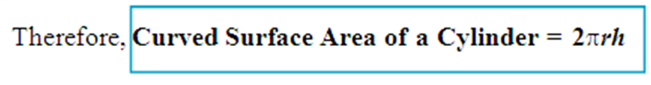
Where r is the radius of the base of the cylinder and h is the height of the cylinder.
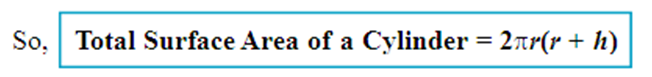
Where h is the height of the cylinder and r its radius.
Surface Area of a Right Circular Cone
- Books Name
- Kaysons Academy Maths Foundation Book
- Publication
- Kaysons Publication
- Course
- JEE
- Subject
- Maths
Surface Area of a Right Circular Cone
So, far have been generating solids by stacking up congruent figures. Incidentally, such figures are called prisms. Now let us look at another kind of solid which is not a prism. (These kinds of solids are called pyramids). Let us see how we can generate them.
Activity: Cut out a right-angled triangle ABC right angled at B. Paste a long thick string along one of the perpendicular sides say AB of the triangle [see Fig (a)]. Hold the string with your hands on either sides of the triangle and rotate the triangle about the string a number of times. What happens? Do you recognize the shape that the triangle is forming as it rotates around the string [see Fig (b)] Does it remind you of the time you had eaten an ice-cream heaped into a container of that shape [see Fig (c) and (d)]?
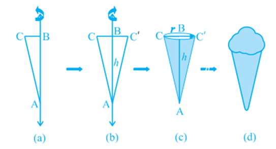
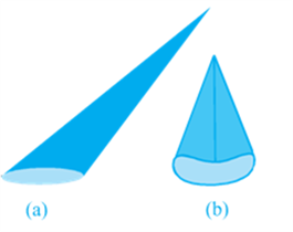
This is called a right circular cone. In Fig (c) of the right circular cone, the point A is called the vertex, AB is called the height, BC is called the radius and AC is called the slant height of the cone. Here B will be the centre of circular base of the cone. The height, radius and slant height of the cone are usually denoted by h, r and l respectively. Once again, let us see what kind of cone we can not call a right circular cone. Here, you are (see Fig)! What you see in these figures are not right circular cones; because in (a), the line joining its vertex to the centre of its base is not at right angle to the base, and in (b) the base is not circular.
As in the case of cylinder, since we will be studying only about right circular cones, remember that by ‘cone’ in this chapter, we shall mean a ‘right circular cone.’
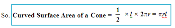
Where r is its base radius and l its slant height.
Surface Area of a Sphere
- Books Name
- Kaysons Academy Maths Foundation Book
- Publication
- Kaysons Publication
- Course
- JEE
- Subject
- Maths
Surface Area of a Sphere
What is a sphere? Is it the same as a circle? Can you draw a circle on a paper? Yes, you can, because a circle is a plane closed figure whose every point lies at a constant distance (called radius) from a fixed point, which is called the centre of the circle. Now if you paste a string along a diameter of a circular disc and rotate it as you had rotated the triangle in the previous section, you see a new solid (see Fig). What does it resemble? A ball? Yes. It is called a sphere.
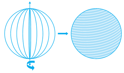
Can you guess what happens to the centre of the circle, when it forms a sphere on rotation? Of course, it becomes the centre of the sphere. So, a sphere is a three dimensional figure (solid figure), which is made up of all points in the space,
which lie at a constant distance called the radius, from a fixed point called the centre of the sphere.
The string, which had completely covered the surface area of the sphere, has been used to completely fill the regions of four circles, all of the same radius as of the sphere.
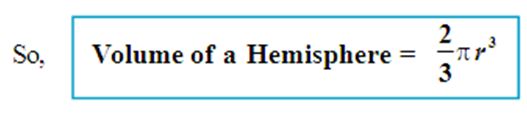
So, what does that mean? This suggests that the surface area of a sphere of radius
r = 4 times the area of a circle of radius r = 4 = × (πr2)
Where r is the radius of the sphere,
![]()
Where r is the radius of the sphere of which the hemisphere is a part.
Now taking the two faces of a hemisphere, its surface ![]()
Volume of a Cuboid
- Books Name
- Kaysons Academy Maths Foundation Book
- Publication
- Kaysons Publication
- Course
- JEE
- Subject
- Maths
Volume of a Cuboid
You have already learnt about volumes of certain figures (objects) in earlier classes. Recall that solid objects occupy space. The measure of this occupied space is called the Volume of the object.
Note: If an object is solid, then the space occupied by such an object is measured, and is termed the Volume of the object. On the other hand, if the object is hollow, then interior is empty, and can be filled with air, or some liquid that will take the shape of its container. In this case, the volume of the substance that can fill the interior is called the capacity of the container. In short, the volume of an object is the measure of the space it occupies, and the capacity of an object is the volume of substance its interior can accommodate. Hence, the unit of measurement of either of the two is cubic unit.
So, if we were to talk of the volume of a cuboid, we would be considering the measure of the space occupied by the cuboid.
Further, the area or the volume is measured as the magnitude of a region. So, correctly speaking, we should be finding the area of a circular region, or volume of a cuboidal region, or volume of a spherical region, etc. But for the sake of simplicity, we say, find the area of a circle, volume of a cuboid or a sphere even though these mean only their boundaries.
Observe Fig. Suppose we say that the area of each rectangle is A, the height up to which the rectangles are stacked is h and the volume of the cuboid is V. Can you tell what would be the relationship between V, A and h?
The area of the plane region occupied by each rectangle × height
= Measure of the space occupied by the cuboid
So, we get A × h = V

or l × b × h, where l, b and h are respectively the length, breadth and height of the cuboid.
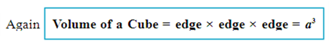
Where a is the edge of the cube (see Fig).
So, if a cube has edge of 12 cm,
then volume of the cube = 12 × 12 × 12 cm3
= 1728 cm3.
Recall that you have learnt these formulae in earlier classes. Now let us take some examples to illustrate the use of these formulae:
Volume of a Cylinder and Volume of a Right Circular Cone
- Books Name
- Kaysons Academy Maths Foundation Book
- Publication
- Kaysons Publication
- Course
- JEE
- Subject
- Maths
Volume of a Cylinder Volume of a Right Circular Cone
Just as a cuboid is built up with rectangles of the same size, we have seen that a right circular cylinder can be built up using circles of the same size. So, using the same argument as for a cuboid, we can see that the volume of a cylinder can be obtained as:
base area × height = area of circular base × height = πr2h
![]()
Where r is the base radius and h is the height of the cylinder.
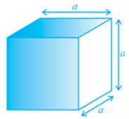
In Fig, can you see that there is a right circular cylinder and a right circular cone of the same base radius and the same height?
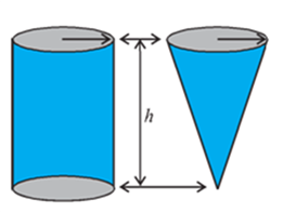
Activity: Try to make a hollow cylinder and a hollow cone like this with the same base radius and the same height (see Fig). Then, we can try out an experiment that will help us, to see practically what the volume of a right circular cone would be!
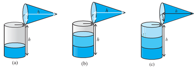
So, let us start like this.
Fill the cone up to the brim with sand once, and empty it into the cylinder. We find that it fills up only a part of the cylinder [see Fig (a)].
When we fill up the cone again to the brim, and empty it into the cylinder, we see that the cylinder is still not full [see Fig (b)].
When the cone is filled up for the third time, and emptied into the cylinder, it can be seen that the cylinder is also full to the brim [see Fig (c)].
With this, we can safely come to the conclusion that three times the volume of a cone, makes up the volume of a cylinder, which has the same base radius and the same height as the cone, which means that the volume of the cone is one-third the volume of the cylinder.
Where r is the base radius and h is the height of the cone.
Volume of a sphere
- Books Name
- Kaysons Academy Maths Foundation Book
- Publication
- Kaysons Publication
- Course
- JEE
- Subject
- Maths
Volume of a sphere
Now, let us see how to go about measuring the volume of a sphere. First, take two or three spheres of different radii, and a container big enough to be able to put each of the spheres into it, one at a time. Also, take a large trough in which you can place the container. Then, fill the container up to the brim with water [see Fig (a)].
Now, carefully place one of the spheres in the container. Some of the water from the container will over flow into the trough in which it is kept [see Fig (b)]. Carefully pour out the water from the trough into a measuring cylinder (i.e., a graduated cylindrical jar) and measure the water over flowed [see Fig (c)]. Suppose the radius of the immersed sphere is r (you can find the radius by measuring the diameter of the sphere).
Then evaluate ![]() Do you find this value almost equal to the measure of the volume over flowed?
Do you find this value almost equal to the measure of the volume over flowed?
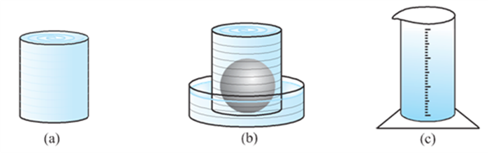
Once again repeat the procedure done just now, with a different size of sphere.
Find the radius R of this sphere and then calculate the value of ![]() Once again this
Once again this
value is nearly equal to the measure of the volume of the water displaced (over flowed)
by the sphere. What does this tell us? We know that the volume of the sphere is the same as the measure of the volume of the water displaced by it. By doing this experiment repeatedly with spheres of varying radii, we are getting the same result,
namely, the volume of a sphere is equal to ![]() times the cube of its radius. This gives us the idea that
times the cube of its radius. This gives us the idea that
Where r is the radius of he sphere.
Later, in higher classes it can be proved also. But at this stage, we will just take it as true.
Since a hemisphere is half of a sphere, can you guess what the volume of a hemisphere will be? Yes. It is ![]()
Where r is the radius of the hemisphere.
Let us take some examples to illustrate the use of these formulae.
Congruence of Triangles and Criteria for Congruence of Triangles
- Books Name
- Kaysons Academy Maths Foundation Book
- Publication
- Kaysons Publication
- Course
- JEE
- Subject
- Maths
Chapter-6
Triangles
Congruence of Triangles
You must have observed that two copies of your photographs of the same size are identical. Similarly, two bangles of the same size, two ATM cards issued by the same bank are identical. You may recall that on placing a one rupee coin on another minted in the same year, they cover each other completely.
Do you remember what such figures are called? Indeed they are called congruent figures (‘congruent’ means equal in all respects or figures whose shapes and sizes are both the same).
Now, draw two circles of the same radius and place one on the other. What do you observe? They cover each other completely and we call them as congruent circles.

You may wonder why we are studying congruence. You all must have seen the ice tray in your refrigerator. Observe that the moulds for making ice are all congruent. The cast used for moulding in the tray also has congruent depressions (may be all are rectangular or all circular or all triangular). So, whenever identical objects have to be produced, the concept of congruence is used in making the cast.
Sometimes, you may find it difficult to replace the refill in your pen by a new one and this is so when the new refill is not of the same size as the one you want to remove. Obviously, if the two refills are identical or congruent, the new refill fits.
So, you can find numerous examples where congruence of objects is applied in daily life situations.
Can you think of some more examples of congruent figures?
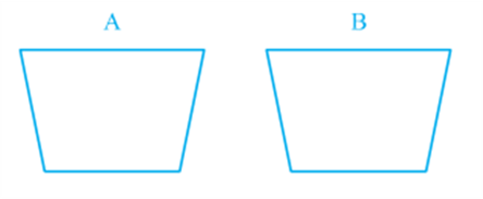
Now, which of the following figures are not congruent to the square in
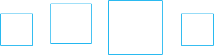
The large squares (ii) and (iii) are obviously not congruent to the one in
(i), but the square (iv) is congruent to the one given.
Let us now discuss the congruence of two triangles.
You already know that two triangles are congruent if the sides and angles of one triangle are equal to the corresponding sides and angles of the other triangle.
Now, which of the triangles given below are congruent to triangle ABC
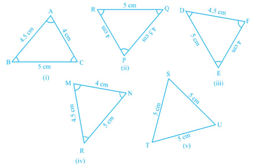
Cut out each of these triangles from Fig. (ii) to (v) and turn them around and try to cover Δ ABC. Observe that triangles in Fig. 7.4 (ii), (iii) and (iv) are congruent to Δ ABC while Δ TSU of Fig 7.4 (v) is not congruent to Δ ABC.
If Δ PQR is congruent to Δ ABC, we write Δ PQR ≅ Δ ABC.
Notice that when Δ PQR ≅ Δ ABC, then sides of Δ PQR fall on corresponding equal sides of Δ ABC and so is the case for the angles.
That is, PQ covers AB, QR covers BC and RP covers CA; ∠ P covers ∠ A,
∠ Q covers ∠ B and ∠ R covers ∠ C. Also, there is a one-one correspondence
Between the vertices. That is, P corresponds to A, Q to B, R to C and so on which is written as
P ↔ A, Q ↔ B, R ↔ C
Note that under this correspondence, Δ PQR ≅ Δ ABC; but it will not be correct to write ΔQRP ≅ Δ ABC.
Similarly, for
FD ↔ AB, DE ↔ BC and EF ↔ CA
and F ↔ A, D ↔ B and E ↔ C
So, Δ FDE ≅ Δ ABC but writing Δ DEF ≅ Δ ABC is not correct.
Give the correspondence between the triangle in Fig. 7.4 (iv) and Δ ABC.
So, it is necessary to write the correspondence of vertices correctly for writing of congruence of triangles in symbolic form.
Note that in congruent triangles corresponding parts are equal and we write in short ‘CPCT’ for corresponding parts of congruent triangles .
Now, draw two triangles with one side 4 cm and one angle 50°. Are they congruent?
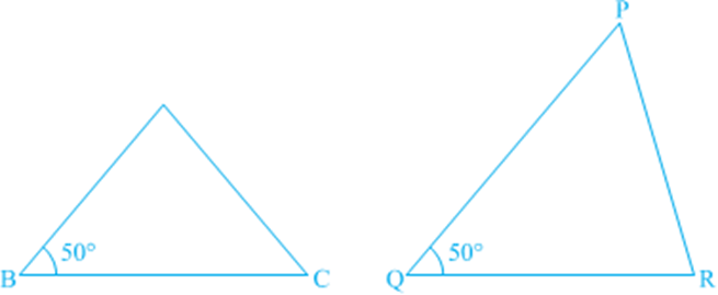
See that these two triangles are not congruent.
Repeat this activity with some more pairs of triangles.
So, equality of one pair of sides or one pair of sides and one pair of angles is not sufficient to give us congruent triangles.
What would happen if the other pair of arms (sides) of the equal angles are also equal?
BC = QR, ∠ B = ∠ Q and also, AB = PQ. Now, what can you say
about congruence of Δ ABC and Δ PQR?
Recall from your earlier classes that, in this case, the two triangles are congruent.
Verify this for Δ ABC and Δ PQR
Repeat this activity with other pairs of triangles. Do you observe that the equality of two sides and the included angle is enough for the congruence of triangles? Yes, it is enough.
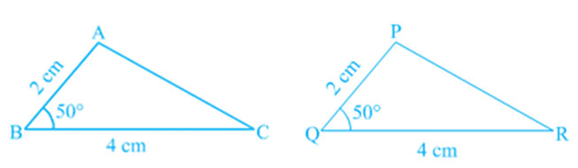
This is the first criterion for congruence of triangles.
Axiom 7.1 (SAS congruence rule) : Two triangles are congruent if two sides and the included angle of one triangle are equal to the two sides and the included angle of the other triangle.
This result cannot be proved with the help of previously known results and so it is accepted true as an axiom (see Appendix 1).
Let us now take some examples.
Theorems
- Books Name
- Kaysons Academy Maths Foundation Book
- Publication
- Kaysons Publication
- Course
- JEE
- Subject
- Maths
Theorem
Theorem 7.1 (ASA congruence rule) : Two triangles are congruent if two angles and the included side of one triangle are equal to two angles and the included side of other triangle.
So, two triangles are congruent if any two pairs of angles and one pair of corresponding sides are equal. We may call it as the AAS Congruence Rule.
Some Properties of a Triangle
In the above section you have studied two criteria for congruence of triangles. Let us now apply these results to study some properties related to a triangle whose two sides are equal.
Perform the activity given below:
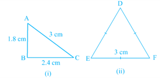
Construct a triangle in which two sides are equal, say each equal to 3.5 cm and the third side equal to 5 cm. You have done such constructions in earlier classes
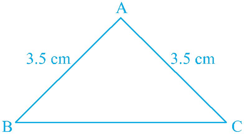
Do you remember what is such a triangle called?
A triangle in which two sides are equal is called an isosceles triangle . So, Δ ABC
an isosceles triangle with AB = AC.
Now, measure ∠ B and ∠ C. What do you observe?
Repeat this activity with other isosceles triangles with different sides.
You may observe that in each such triangle, the angles opposite to the equal sides are equal.
This is a very important result and is indeed true for any isosceles triangle. It can be proved as shown below.
Theorem 7.2: Angles opposite to equal sides of an isosceles triangle are equal.
This result can be proved in many ways. One of the proofs is given here.
Theorem 7.3: The sides opposite to equal angles of a triangle are equal.
This is the converse of Theorem 7.2.
You can prove this theorem by ASA congruence rule.
Let us take some examples to apply these results.
Some More Criteria for Congruence of Triangles
You have seen earlier in this chapter that equality of three angles of one triangle to three angles of the other is not sufficient for the congruence of the two triangles. You may wonder whether equality of three sides of one triangle to three sides of another triangle is enough for congruence of the two triangles. You have already verified in earlier classes that this is indeed true.
To be sure, construct two triangles with sides 4 cm, 3.5 cm and 4.5 cm. Cut them out and place them on each other. What do you observe? They cover each other completely, if the equal sides are placed on each other. So, the triangles are congruent.
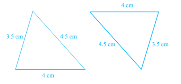
Repeat this activity with some more triangles. We arrive at another rule for congruence.
Theorem 7.4 (SSS congruence rule) : If three sides of one triangle are equal to the three sides of another triangle, then the two triangles are congruent.
This theorem can be proved using a suitable construction.
You have already seen that in the SAS congruence rule, the pair of equal angles has to be the included angle between the pairs of corresponding pair of equal sides and if this is not so, the two triangles may not be congruent.
Perform this activity:
Construct two right angled triangles with hypotenuse equal to 5 cm and one side equal to 4 cm each
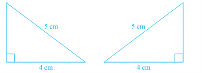
Cut them out and place one triangle over the other with equal side placed on each other. Turn the triangles, if necessary. What do you observe?
The two triangles cover each other completely and so they are congruent. Repeat this activity with other pairs of right triangles. What do you observe?
You will find that two right triangles are congruent if one pair of sides and the hypotenuse are equal. You have verified this in earlier classes.
Note that, the right angle is not the included angle in this case.
So, you arrive at the following congruence rule:
Theorem 7.5 (RHS congruence rule): If in two right triangles the hypotenuse and one side of one triangle are equal to the hypotenuse and one side of the other triangle, then the two triangles are congruent.
Note that RHS stands for Right angle - Hypotenuse - Side.
Let us now take some examples.
Inequalities in a Triangle
- Books Name
- Kaysons Academy Maths Foundation Book
- Publication
- Kaysons Publication
- Course
- JEE
- Subject
- Maths
Inequalities in a Triangle
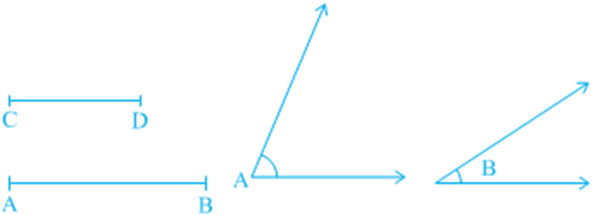
So far, you have been mainly studying the equality of sides and angles of a triangle or triangles. Sometimes, we do come across unequal objects, we need to compare them. For example, line-segment AB is greater in length as compared to line segment CD (i) and ∠ A is greater than ∠ B
Let us now examine whether there is any relation between unequal sides and unequal angles of a triangle. For this, let us perform the following activity:
Activity: Fix two pins on a drawing board say at B and C and tie a thread to mark a side BC of a triangle.
Fix one end of another thread at C and tie a pencil at the other (free) end . Mark a point A with the pencil and draw Δ ABC. Now, shift the pencil and mark another point A′ on CA beyond A (new position of it)
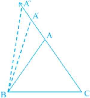
So, A′C > AC (Comparing the lengths) Join A′ to B and complete the triangle A′BC.
What can you say about ∠ A′BC and ∠ ABC? Compare them. What do you observe?
Clearly, ∠ A′BC > ∠ ABC
Continue to mark more points on CA (extended) and draw the triangles with the side BC and the points marked.
You will observe that as the length of the side AC is increased (by taking different positions of A), the angle opposite to it, that is, ∠ B also increases.
Let us now perform another activity:
Activity: Construct a scalene triangle (that is a triangle in which all sides are of different lengths). Measure the lengths of the sides.
Now, measure the angles. What do you observe?
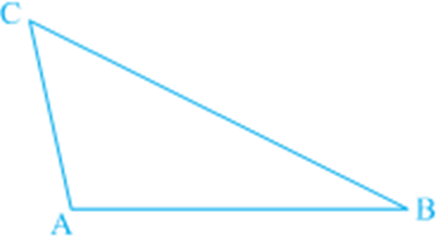
In Δ ABC of BC is the longest side and AC is the shortest side.
Also, ∠ A is the largest and ∠ B is the smallest.
Repeat this activity with some other triangles.
We arrive at a very important result of inequalities in a triangle. It is stated in the form of a theorem as shown below:
Figures on the Same Base and Between the Same Parallels
- Books Name
- Kaysons Academy Maths Foundation Book
- Publication
- Kaysons Publication
- Course
- JEE
- Subject
- Maths
Chapter -9
Areas Of Parallelograms And Triangles
You may recall that the part of the plane enclosed by a simple closed figure is called a planar region corresponding to that figure. The magnitude or measure of this planar region is called its area. This magnitude or measure is always expressed with the help of a number (in some unit) such as 5 cm2, 8 m2, 3 hectares etc. So, we can say that area of a figure is a number (in some unit) associated with the part of the plane enclosed by the figure.
We are also familiar with the concept of congruent figures from earlier classes and from Chapter 7. Two figures ar e called congruent, if they have the same shape and the same size. In other words, if two figures A and B are congruent (see Fig), then using a tracing paper,
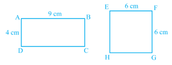
You can superpose one figure over the other such that it will cover the other completely. So if two figures A and B are congruent, they must have equal areas. However, the converse of this statement is not true. In other words, two figures having equal areas need not be congr uent. For example, in Fig, rectangles ABCD and EFGH have equal areas (9 × 4 cm2 and 6 × 6 cm2) but clearly they are not congruent. (Why?)
Now let us look at Fig. given below:

You may observe that planar region formed by figure T is made up of two planar regions formed by figures P and Q. You can easily see that
Area of figure T = Area of figure P + Area of figure Q.
You may denote the area of figure A as ar(A), area of figure B as ar(B), area of figure T as ar(T), and so on. Now you can say that area of a figure is a number (in some unit) associated with the part of the plane enclosed by the figure with the following two properties:
(1) If A and B are two congruent figures, then ar(A) = ar(B);
and (2) if a planar region formed by a figure T is made up of two non-overlapping planar regions formed by figures P and Q, then ar(T) = ar(P) + ar(Q).
You are also aware of some formulae for finding the areas of different figures such as rectangle, square, parallelogram, triangle etc., from your earlier classes. In this chapter, attempt shall be made to consolidate the knowledge about these formulae by studying some relationship between the areas of these geometric figures under the condition when they lie on the same base and between the same parallels. This study will also be useful in the understanding of some results on ‘similarity of triangles’.
Figures on the Same Base and Between the Same Parallels
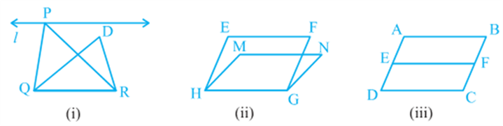
Look at the following figures:
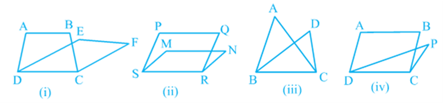
In Fig (i), trapezium ABCD and parallelogram EFCD have a common side DC. We say that trapezium ABCD and parallelogram EFCD are on the same base DC. Similarly, in Fig (ii), parallelograms PQRS and MNRS are on the same base SR; in Fig (iii), triangles ABC and DBC are on the same base BC and in Fig (iv), parallelogram ABCD and triangle PDC are on the same base DC.
Now look at the following figures:
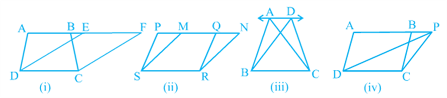
In Fig (i), clearly trapezium ABCD and parallelogram EFCD are on the same base DC. In addition to the above, the vertices A and B (of trapezium ABCD) opposite to base DC and the vertices E and F (of parallelogram EFCD) opposite to base DC lie on a line AF parallel to DC. We say that trapezium ABCD and parallelogram EFCD are on the same base DC and between the same parallels AF and DC. Similarly, parallelograms PQRS and MNRS are on the same base SR and between the same parallels PN and SR [see Fig (ii)] as vertices P and Q of PQRS and vertices M and N of MNRS lie on a line PN parallel to base SR. In the same way, triangles ABC and DBC lie on the same base BC and between the same parallels AD and BC [see Fig (iii)] and parallelogram ABCD and triangle PCD lie on the same base DC and between the same parallels AP and DC [see Fig (iv)].
So, two figures are said to be on the same base and between the same parallels, if they have a common base (side) and the vertices (or the vertex) opposite to the common base of each figure lie on a line parallel to the base. Keeping in view the above statement, you cannot say that Δ PQR and Δ DQR of Fig (i) lie between the same parallels l and QR. Similarly, you cannot say that
Parallelograms EFGH and MNGH of Fig (ii) lie between the same parallels EF and HG and that parallelograms ABCD and EFCD of Fig (iii) lie between the same parallels AB and DC (even though they have a common base DC and lie between the parallels AD and BC). So, it should clearly be noted that out of the two parallels, one must be the line containing the common base. Note that ΔABC and ΔDBE of Fig (i) are not on the common base. Similarly, ΔABC and parallelogram PQRS of Fig (ii) are also not on the same base.
Parallelograms on the same Base and Between the same Parallels
- Books Name
- Kaysons Academy Maths Foundation Book
- Publication
- Kaysons Publication
- Course
- JEE
- Subject
- Maths
Parallelograms on the same Base and Between the same Parallels
Now let us try to find a relation, if any, between the areas of two parallelograms on the same base and between the same parallels. For this, let us perform the following activities:
Activity 1: Let us take a graph sheet and draw two parallelograms ABCD and PQCD on it as shown in Fig.
The above two parallelograms are on the same base DC and between the same parallels PB and DC. You may recall the method of finding the areas of these two parallelograms by counting the squares.
In this method, the area is found by counting the number of complete squares enclosed by the figure, the number of squares a having more than half their parts enclosed by the figure and the number of squares having half their parts enclosed by the figure. The squares whose less than half parts are enclosed by the figure are ignored. You will find that areas of both the parallelograms are (approximately) 15cm2. Repeat this activity* by drawing some more pairs of parallelograms on the graph sheet. What do you observe? Are the areas of the two parallelograms different or equal? If fact, they are equal. So, this may lead you to conclude that parallelograms on the same base and between the same parallels are equal in area. However, remember that this is just a verification.
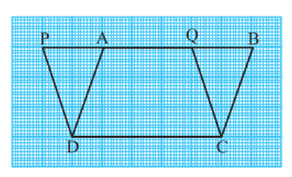
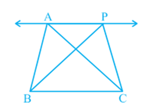
Triangles on the same Base and between the same Parallels
Let us look at Fig. In it, you have two triangles ABC and PBC on the same base BC and between the same parallels BC and AP. What can you say about the areas of such triangles? To answer this question, you may perform the activity of drawing several pairs of triangles on the same base and between the same parallels on the graph sheet and find their areas by the method of counting the squares. Each time, you will find that the areas of the two triangles are (approximately) equal. This activity can be performed using a geoboard also. You will again find that the two areas are (approximately) equal.
To obtain a logical answer to the above question, you may proceed as follows:
In Fig, draw CD || BA and CR || BP such that D and R lie on line AP (see Fig).
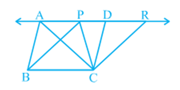
From this, you obtain two parallelograms PBCR and ABCD on the same base BC and between the same parallels BC and AR.
![]()
![]()
![]()
![]()
In this way, you have arrived at the following theorem:
Theorem: Two triangles on the same base (or equal bases) and between the same parallels are equal in area.
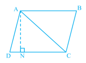
Now, suppose ABCD is a parallelogram whose one of the diagonals is AC (see Fig).
Let AN ⊥ DC. Note that
![]()
![]()
![]()
![]()
![]()
Circles and Its Related Terms: A Review
- Books Name
- Kaysons Academy Maths Foundation Book
- Publication
- Kaysons Publication
- Course
- JEE
- Subject
- Maths
Chapter -10
Circles
Circles and Its Related Terms: A Review
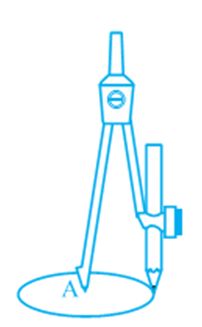
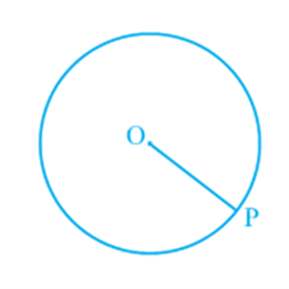
Take a compass and fix a pencil in it. Put its pointed leg on a point on a sheet of a paper. Open the other leg to some distance. Keeping the pointed leg on the same point, rotate the other leg through one revolution. What is the closed figure traced by the pencil on paper? As you know, it is a circle (see Fig). How did you get a circle? You kept one point fixed (A in Fig) and drew all the points that were at a fixed distance from A. This gives us the following definition:
The collection of all the points in a plane, which are at a fixed distance from a fixed point in the plane, is called a circle.
The fixed point is called the centre of the circle and the fixed distance is called the radius of the circle. In Fig, O is the centre and the length OP is the radius of the circle.
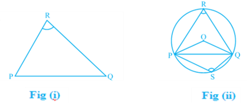
Angle Subtended by a Chord at a Point Take a line segment PQ and a point R not on the line containing PQ. Join PR and QR (see Fig (i)). Then ∠ PRQ is called the angle subtended by the line segment PQ at the point R. What are angles POQ, PRQ and PSQ called in Fig (ii)? ∠ POQ is the angle subtended by the chord PQ at the centre O, ∠ PRQ and ∠ PSQ are respectively the angles subtended by PQ at points R and S on the major and minor arcs PQ.
Let us examine the relationship between the size of the chord and the angle subtended by it at the centre. You may see by drawing different chords of a circle and angles subtended by them at the centre that the longer is the chord, the bigger will be the angle subtended by it at the centre. What will happen if you take two equal chords of a circle? Will the angles subtended at the centre be the same or not?
Draw two or more equal chords of a circle and measure the angles subtended by them at the centre (see Fig). You will find that the angles subtended by them at the centre are equal. Let us give a proof of this fact.
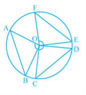
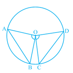
Theorem: Equal chords of a circle subtend equal angles at the centre.
Proof: You are given two equal chords AB and CD of a circle with centre O (see Fig). You want to prove that ∠ AOB = ∠ COD. In triangles AOB and COD,
In triangles AOB and COD,
OA = O C (Radii of a circle)
OB = OD (Radii of a circle)
AB = C D (Given)
Therefore, Δ AOB ≅ Δ COD (SSS rule)
This gives ∠ AOB = ∠ COD
(Corresponding parts of congruent triangles).
Which is denoted by R.? Therefore, a real number is either rational or irrational. So, we can say that every real number is represented by a unique point on the number line. Also, every point on the number line represents a unique real number. This is why we call the number line, the real number line.
A circle divides the plane on which it lies into three parts. They are: (i) inside the circle, which is also called the interior of the circle; (ii) the circle and (iii) outside the circle, which is also called the exterior of the circle (see Fig). The circle and its interior make up the circular region.
Perpendicular from the Centre to a Chord
- Books Name
- Kaysons Academy Maths Foundation Book
- Publication
- Kaysons Publication
- Course
- JEE
- Subject
- Maths
Perpendicular from the Centre to a Chord
Activity: Draw a circle on a tracing paper. Let O be its centre. Draw a chord AB. Fold the paper along a line through O so that a portion of the chord falls on the other. Let the crease cut AB at the point M. Then, ∠ OMA = ∠ OMB = 90° or OM is perpendicular to AB. Does the point B coincide with A (see Fig)?
Give a proof yourself by joining OA and OB and proving the right triangles OMA and OMB to be congruent. This example is a particular instance of the following result:
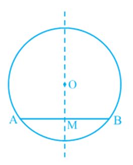
Theorem: The perpendicular from the centre of a circle to a chord bisects the chord.
What is the converse of this theorem? To write this, first let us be clear what is assumed in Theorem and what is proved. Given that the perpendicular from the centre of a circle to a chord is drawn and to prove that it bisects the chord. Thus in the converse, what the hypothesis is ‘if a line from the centre bisects a chord of a circle’ and what is to be proved is ‘the line is perpendicular to the chord’. So the converse is:
Theorem: The line drawn through the centre of a circle to bisect a chord is perpendicular to the chord.
Is this true? Try it for few cases and see. You will see that it is true for these cases. See if it is true, in general, by doing the following exercise. We will write the stages and you give the reasons.
Let AB be a chord of a circle with centre O and O is joined to the mid-point M of AB. You have to prove that OM ⊥ AB. Join OA and OB (see Fig). In triangles OAM and OBM,
OA = O B (Why?)
AM = BM (Why?)
OM = OM (Common)
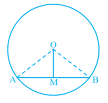
Therefore, ΔOAM ≅ ΔOBM (How?)
This gives ∠OMA = ∠OMB = 90 (Why?)
Circle through Three Points
You have learnt in Chapter 6, that two points are sufficient to determine a line. That is, there is one and only one line passing through two points. A natural question arises. How many points are sufficient to determine a circle?
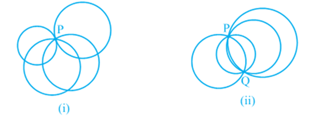
Take a point P. How many circles can be drawn through this point? You see that there may be as many circles as you like passing through this point [see Fig (i)]. Now take two points P and Q. You again see that there may be an infinite number of circles passing through P and Q [see Fig (ii)]. What will happen when you take three points A, B and C? Can you draw a circle passing through three collinear points?
Theorem: There is one and only one circle passing through three given non-collinear points.
Angle Subtended by an Arc of a Circle
You have seen that the end points of a chord other than diameter of a circle cuts it into two arcs – one major and other minor. If you take two equal chords, what can you say about the size of arcs? Is one arc made by first chord equal to the corresponding arc made by another chord? In fact, they are more than just equal in length. They are congruent in the sense that if one arc is put on the other, without bending or twisting, one superimposes the other completely.
You can verify this fact by cutting the arc, corresponding to the chord CD from the circle along CD and put it on the corresponding arc made by equal chord AB. You will find that the arc CD superimpose the arc AB completely (see Fig). This shows that equal chords make congruent arcs and conversely congruent arcs make equal chords of a circle. You can state it as follows:
If two chords of a circle are equal, then their corresponding arcs are congruent and conversely, if two arcs are congruent, then their corresponding chords are equal.
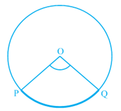
Also the angle subtended by an arc at the centre is defined to be angle subtended by the corresponding chord at the centre in the sense that the minor arc subtends the angle and the major arc subtends the reflex angle. Therefore, in Fig, the angle subtended by the minor arc PQ at O is ∠POQ and the angle subtended by the major arc PQ at O is reflex angle POQ.
In view of the property above and Theorem, the following result is true:
Congruent arcs (or equal arcs) of a circle subtend equal angles at the centre.
Therefore, the angle subtended by a chord of a circle at its centre is equal to the angle subtended by the corresponding (minor) arc at the centre. The following theorem gives the relationship between the angles subtended by an arc at the centre and at a point on the circle.
Cyclic Quadrilaterals
- Books Name
- Kaysons Academy Maths Foundation Book
- Publication
- Kaysons Publication
- Course
- JEE
- Subject
- Maths
Cyclic Quadrilaterals
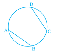
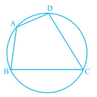
A quadrilateral ABCD is called cyclic if all the four vertices of it lie on a circle (see Fig). You will find a peculiar property in such quadrilaterals. Draw several cyclic quadrilaterals of different sides and name each of these as ABCD. (This can be done by drawing several circles of different radii and taking four points on each of them.) Measure the opposite angles and write your observations in the following table.
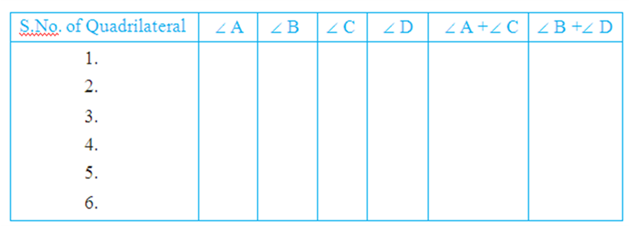
What do you infer from the table?
Theorem: The sum of either pair of opposite angles of a cyclic quadrilateral is 180º.
Theorem: If the sum of a pair of opposite angles of a quadrilateral is 180º, the quadrilateral is cyclic.
Introduction
- Books Name
- Kaysons Academy Maths Foundation Book
- Publication
- Kaysons Publication
- Course
- JEE
- Subject
- Maths
Chapter -4
Introduction To Euclid’s Geometry
Introduction
The word ‘geometry’ comes form the Greek words ‘geo’, meaning the ‘earth’, and ‘metrein’, meaning ‘to measure’. Geometry appears to have originated from the need for measuring land. This branch of mathematics was studied in various forms in every ancient civilisation, be it in Egypt, Babylonia, China, India, Greece, the Incas, etc. The people of these civilisations faced several practical problems which required the development of geometry in various ways.
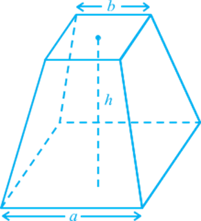
For example, whenever the river Nile overflowed, it wiped out the boundaries between the adjoining fields of different land owners. After such flooding, these boundaries had to be redrawn. For this purpose, the Egyptians developed a number of geometric techniques and rules for calculating simple areas and also for doing simple constructions. The knowledge of geometry was also used by them for computing volumes of granaries, and for constructing canals and pyramids. They also knew the correct formula to find the volume of a truncated pyramid (see Fig.).You know that a pyramid is a solid figure, the base of which is a triangle, or square, or some Other polygon, and its side faces are triangles converging to a point at the top.
Euclid’s Definitions, Axioms and Postulates
The Greek mathematicians of Euclid’s time thought of geometry as an abstract model of the world in which they lived. The notions of point, line, plane (or surface) and so on were derived from what was seen around them. From studies of the space and solids in the space around them, an abstract geometrical notion of a solid object was developed. A solid has shape, size, position, and can be moved from one place to another. Its boundaries are called surfaces. They separate one part of the space from another, and are said to have no thickness. The boundaries of the surfaces are curves or straight lines. These lines end in points.
Consider the three steps from solids to points (solids-surfaces-lines-points). In each step we lose one extension, also called a dimension. So, a solid has three dimensions, a surface has two, a line has one and a point has none. Euclid summarised these statements as definitions. He began his exposition by listing 23 definitions in Book 1 of the ‘Elements’. A few of them are given below:
-
- A point is that which has no part.
- A line is breathless length.
- The ends of a line are points.
- A straight line is a line which lies evenly with the points on itself.
- A surface is that which has length and breadth only.
- The edges of a surface are lines.
- A plane surface is a surface which lies evenly with the straight lines on itself.
Starting with his definitions, Euclid assumed certain properties, which were not to be proved. These assumptions are actually ‘obvious universal truths’. He divided them into two types: axioms and postulates. He used the term ‘postulate’ for the assumptions that were specific to geometry. Common notions (often called axioms), on the other hand, were assumptions used throughout mathematics and not specifically linked to geometry. For details about axioms and postulates, refer to Appendix 1. Some of Euclid’s axioms, not in his order, are given below:(1) Things which are equal to the same thing are equal to one another.
(2) If equals are added to equals, the wholes are equal.
(3) If equals are subtracted from equals, the remainders are equal.
(4) Things which coincide with one another are equal to one another.
(5) The whole is greater than the part.
(6) Things which are double of the same things are equal to one another.
(7) Things which are halves of the same things are equal to one another.
Now let us discuss Euclid’s five postulates. They are :
Postulate 1: A straight line may be drawn from any one point to any other point.
Note that this postulate tells us that at least one straight line passes through two distinct points, but it does not say that there cannot be more than one such line. However, in his work, Euclid has frequently assumed, without mentioning, that there is a unique line joining two distinct points. We state this result in the form of an axiom as follows:
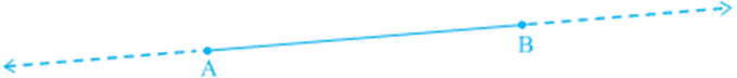
Postulate 2: A terminated line can be produced indefinitely.Note that what we call a line segment now-a-days is what Euclid called a terminated line. So, according to the present day terms, the second postulate says that a line segment can be extended on either side to form a line.
Postulate 3: A circle can be drawn with any centre and any radius.
Postulate 4: All right angles are equal to one another.
Postulate 5: If a straight line falling on two straight lines makes the interior angles on the same side of it taken together less than two right angles, then the two straight lines, if produced indefinitely, meet on that side on which the sum of angles is less than two right angles.
Equivalent Versions of Euclid’s Fifth Postulate
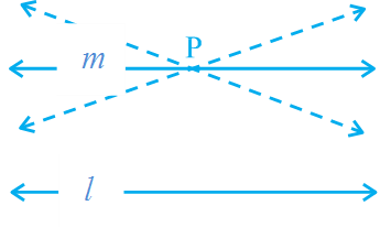
Euclid’s fifth postulate is very significant in the history of mathematics. Recall it again from Section 5.2. We see that by implication, no intersection of lines will take place when the sum of the measures of the interior angles on the same side of the falling line is exactly 180°. There are several equivalent versions of this postulate. One of them is ‘Playfair’s Axiom’ (given by a Scottish mathematician John Playfair in 1729), as stated below: ‘For every line l and for every point P not lying on l, there exists a unique line m passing through P and parallel to l’.
From, you can see that of all the lines passing through the point P, only line m is parallel to line l.
This result can also be stated in the following form:
Two distinct intersecting lines cannot be parallel to the same line.
Introduction
- Books Name
- Kaysons Academy Maths Foundation Book
- Publication
- Kaysons Publication
- Course
- JEE
- Subject
- Maths
Chapter -14
HERON’S FORMULA
Introduction
You have studied in earlier classes about figures of different shapes such as squares, rectangles, triangles and quadrilaterals. You have also calculated perimeters and the areas of some of these figures like rectangle, square etc. For instance, you can find the area and the perimeter of the floor of your classroom.
Let us take a walk around the floor along its sides once; the distance we walk is its perimeter. The size of the floor of the room is its area.
So, if your classroom is rectangular with length 10 m and width 8 m, its perimeter would be 2(10 m + 8 m) = 36 m and its area would be 10 m × 8 m, i.e., 80 m2.
Unit of measurement for length or breadth is taken as metre (m) or centimeter (cm) etc.
Unit of measurement for area of any plane figure is taken as square metre (m2) or square centimeter (cm2) etc.
Suppose that you are sitting in a triangular garden. How would you find its area? From Chapter 9 and from your earlier classes, you know that:
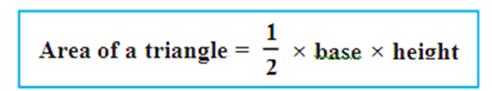
Now suppose we want to find the area of an equilateral triangle PQR with side 10cm (see Fig). To find its area we need its height. Can you find the height of this triangle?
Let us recall how we find its height when we know its sides. This is possible in an Equilateral triangle. Take the mid-point of QR as M and join it to P. We know that PMQ is a right triangle. Therefore, by using Pythagoras Theorem, we can find the length PM as shown below:
![]()
![]()
Therefore, we have PM2 = 75
![]()
![]()
Area of a Triangle – by Heron’s Formula
Heron was born in about 10AD possibly in Alexandria
in Egypt. He worked in applied mathematics. His works
on mathematical and physical subjects are so numerous
and varied that he is considered to be an encyclopedic
writer in these fields. His geometrical works deal largely
with problems on menstruation written in three books.
Book I deals with the area of squares, rectangles, triangles,
trapezoids (trapezium), various other specialized quadrilaterals, the regular polygons, circles, surfaces of cylinders, cones, spheres etc. In this book, Heron has derived the famous formula for the area of a triangle in terms of its three sides.
The formula given by Heron about the area of a triangle is also known as Hero’s formula. It is started as:
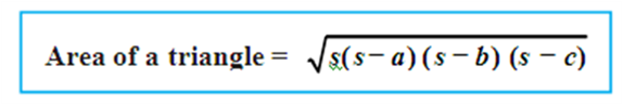
Where a, b and c are the sides of the triangle, and so = semi-perimeter, i.e., half the perimeter of the triangle ![]() .
.
Application of Heron’s Formula in Finding Areas of Quadrilaterals
Suppose that a farmer has a land to be cultivated and she employs some laborers for this purpose on the terms of wages calculated by area cultivated per square meter. How will she do this? Many a time, the fields are in the shape of quadrilaterals. We need to divide the quadrilateral in triangular parts and then use the formula for area of the triangle.
Linear Equations
- Books Name
- Kaysons Academy Maths Foundation Book
- Publication
- Kaysons Publication
- Course
- JEE
- Subject
- Maths
Chapter -7
Linear Equations In Two Variables
Introduction
In earlier classes, you have studied linear equations in one variable. Can you write down a linear equation in one variable? You may say that x + 1 = 0, x + √2 = 0 and √2 y+√3=0 are examples of linear equations in one variable. You also know that such equations have a unique (i.e., one and only one) solution. You may also remember how to represent the solution on a number line. In this chapter, the knowledge of linear equations in one variable shall be recalled and extended to that of two variables. You will be considering questions like: Does a linear equation in two variables have a solution? If yes, is it unique? What does the solution look like on the Cartesian plane? You shall also use the concepts you studied in Chapter 3 to answer these questions.
Linear Equations
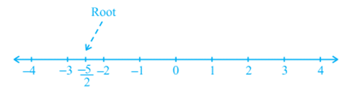
Let us first recall what you have studied so far. Consider the following equation:
2x + 5 = 0
Its solution, i.e., the root of the equation, is – 5/2. This can be represented on the number line as shown below:
While solving an equation, you must always keep the following points in mind: The solution of a linear equation is not affected when:
(i) The same number is added to (or subtracted from) both the sides of the equation.
(ii)You multiply or divide both the sides of the equation by the same non-zero number.
Let us now consider the following situation:
In a One-day International Cricket match between India and Sri Lanka played in Nagpur, two Indian batsmen together scored 176 runs. Express this information in the form of an equation.
Here, you can see that the score of neither of them is known, i.e., there are two unknown quantities. Let us use x and y to denote them. So, the number of runs scored by one of the batsmen is x, and the number of runs scored by the other is y.
We know that
x + y = 176,
Which is the required equation?
This is an example of a linear equation in two variables. It is customary to denote the variables in such equations by x and y, but other letters may also be used. Some examples of linear equations in two variables are:
2s + 3t = 5, p + 4q = 7, πu + 5v = 9 and 3=√2 x-7y.
Note that you can put these equations in the form 1.2s + 3t – 5 = 0,
P + 4q – 7 = 0, πu + 5v – 9 = 0 and ![]()
So, any equation which can be put in the form ax + by + c = 0, where a, b and c are real numbers, a and b are not
both zero, is called a linear equation in two variables.
This means that you can think of many such equations.
Solution of a Linear Equation
You have seen that every linear equation in one variable has a unique solution. What can you say about the solution of a linear equation involving two variables? As there are two variables in the equation, a solution means a pair of values, one for x and one for y which satisfy the given equation. Let us consider the equation 2 x + 3y = 12. Here, x = 3 and y = 2 is a solution because when you substitute x = 3 and y = 2 in the equation above, you find that
2x + 3y = (2 × 3) + (3 × 2) = 12
This solution is written as an ordered pair (3, 2), first writing the value for x and then the value for y. Similarly, (0, 4) is also a solution for the equation above.
On the other hand, (1, 4) is not a solution of 2x + 3y = 12, because on putting x = 1 and y = 4 we get 2x + 3y = 14, which is not 12. Note that (0, 4) is a solution but not (4, 0).
You have seen at least two solutions for 2x + 3y = 12, i.e., (3, 2) and (0, 4). Can you find any other solution? Do you agree that (6, 0) is another solution? Verify the same. In fact, we can get many many solutions in the following way. Pick a value of your choice for x (say x = 2) in 2x + 3y = 12. Then the equation reduces to 4 + 3 y = 12,
Which is a linear equation in one variable. On solving this, you get y=8/3.so (2,8/3) is another solution of 2x + 3y = 12. This gives y=22/3.So,(-5,22/3) is another solution of 2x + 3y = 12. So there is no end to different solutions of a linear equation in two variables. That is, a linear equation in two variables has infinitely many solutions.
Graph of a Linear Equation in Two Variables
- Books Name
- Kaysons Academy Maths Foundation Book
- Publication
- Kaysons Publication
- Course
- JEE
- Subject
- Maths
Graph of a Linear Equation in Two Variables
So far, you have obtained the solutions of a linear equation in two variables algebraically. Now, let us look at their geometric representation. You know that each such equation has infinitely many solutions. How can we show them in the coordinate plane? You may have got some indication in which we write the solution as pairs of values. The solutions of the linear equation in Example 3, namely,
x + 2y = 6
Can be expressed in the form of a table as follows by writing the values of y below the corresponding values of x:
|
x |
0 |
2 |
4 |
6 |
. . . |
|
y |
3 |
2 |
1 |
0 |
. . . |
In the previous chapter, you studied how to plot the points on a graph paper. Let us plot the points (0, 3), (2, 2), (4, 1) and (6, 0) on a graph paper. Now join any two of these points and obtain a line. Let us call this as line AB (see Fig).
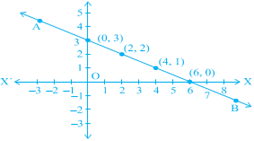
Do you see that the other two points also lie on the line AB? Now, pick another point on this line, say (8, –1). Is this a solution? In fact, 8 + 2(–1) = 6. So, (8, –1) is a solution. Pick any other point on this line AB and verify whether its coordinates satisfy the equation or not. Now, take any point not lying on the line AB, say (2, 0). Do its coordinates satisfy the equation? Check, and see that they do not.
Let us list our observations:
Every point whose coordinates satisfy Equation (1) lies on the line AB.
Every point (a, b) on the line AB gives a solution x = a, y = b of Equation (1).
Any point, which does not lie on the line AB, is not a solution of Equation (1).
So, you can conclude that every point on the line satisfies the equation of the line and every solution of the equation is a point on the line. In fact, a linear equation in two variables is represented geometrically by a line whose points make up the collection of solutions of the equation. This is called the graph of the linear equation. So, to obtain the graph of a linear equation in two variables, it is enough to plot two points corresponding to two solutions and join them by a line. However, it is advisable to plot more than two such points so that you can immediately check the correctness of the graph.
Basic Terms and Definitions
- Books Name
- Kaysons Academy Maths Foundation Book
- Publication
- Kaysons Publication
- Course
- JEE
- Subject
- Maths
Chapter -5
Lines And Angles
Basic Terms and Definitions
Recall that a part (or portion) of a line with two end points is called a line-segment and a part of a line with one end point is called a ray. Note that the line segment AB is denoted by AB, and its length is denoted by AB. The ray AB is denoted by AB , and a line is denoted by AB . However, we will not use these symbols, and will denote the line segment AB, ray AB, length AB and line AB by the same symbol, AB. The meaning will be clear from the context. Sometimes small letters l , m, n, etc. will be used to denote lines.
If three or more points lie on the same line, they are called collinear points; otherwise they are called non-collinear points.
Recall that an angle is formed when two rays originate from the same end point. The rays making an angle are called the arms of the angle and the end point is called the ver. tax of the angle. You have studied different types of angles, such as acute angle, right angle, obtuse angle, straight angle and reflex angle in earlier classes.
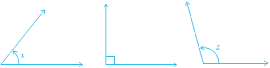
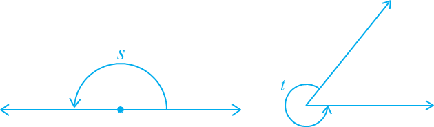
Types of Angles
An acute angle measures between 0° and 90°, whereas a right angle is exactly equal to 90°. An angle greater than 90° but less than 180° is called an obtuse angle. Also, recall that a straight angle is equal to 180°. An angle which is greater than 180° but less than 360° is called a reflex angle. Further, two angles whose sum is 90° are called complementary angles, and two angles whose sum is 180° are called supplementary angles.
You have also studied about adjacent angles in the earlier classes. Two angles are adjacent, if they have a common vertex, a common arm and their non-common arms are on different sides of the common arm. In Fig., ∠ ABD and ∠ DBC are adjacent Angles. Ray BD is their common arm and point B is their common vertex. Ray BA and ray BC are non common arms. Moreover, when two angles are adjacent, then their sum is always equal to the angle formed by the two non- common arms. So, we can write.
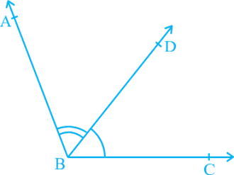
Adjacent angles
∠ ABC = ∠ ABD + ∠ DBC.
Note that ∠ ABC and ∠ ABD are not adjacent angles. Why? Because their non- common arms BD and BC lie on the same side of the common arm BA.
If the non-common arms BA and BC in, form a line then it will look like Fig. 6.3. In this case, ∠ ABD and ∠ DBC are called linear pair of angles.
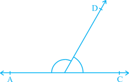
You may also recall the vertically opposite angles formed when two lines, say AB and CD, intersect each other, say at the point O. There are two pairs of vertically opposite angles.
One pair is ∠AOD and ∠BOC. Can you find the other pair?
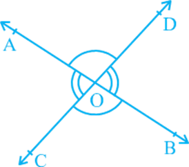
Intersecting Lines and Non-intersecting Lines
Draw two different lines PQ and RS on a paper. You will see that you can draw them in two different ways as shown in Fig.
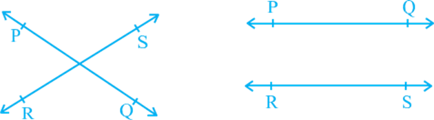
Recall the notion of a line that it extends indefinitely in both directions. Lines PQ and RS in Fig. 6.5 (i) are intersecting lines and in Fig. 6.5 (ii) are parallel lines. Note that the lengths of the common perpendiculars at different points on these parallel lines are the same. This equal length is called the distance between two parallel lines.
Pairs of Angles
In Section 6.2, you have learnt the definitions of some of the pairs of angles such as complementary angles, supplementary angles, adjacent angles, linear pair of angles, etc. Can you think of some relations between these angles? Now, let us find out the relation between the angles formed when a ray stands on a line. Draw a figure in which a ray stands on a line as shown in. Name the line as AB and the ray as OC. What are the angles formed at the point O? They are ∠ AOC, ∠ BOC and ∠ AOB.
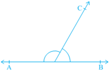
Can we write ∠ AOC + ∠ BOC = ∠ AOB? (1)
Yes! (Why? Refer to adjacent angles in Section 6.2)
What is the measure of ∠ AOB? It is 180°. (Why?) (2)
From (1) and (2), can you say that ∠ AOC + ∠ BOC = 180°? Yes! (Why?)
From the above discussion, we can state the following Axiom:
Axiom 6.1: If a ray stands on a line, then the sum of two adjacent angles so formed is 180°.
Recall that when the sum of two adjacent angles is 180°, then they are called a Linear pair of angles.
In Axiom 6.1, it is given that ‘a ray stands on a line’. From this ‘given’, we have concluded that ‘the sum of two adjacent angles so formed is 180°’. Can we write Axiom 6.1 the other way? That is, take the ‘conclusion’ of Axiom 6.1 as ‘given’ and the ‘given’ as the ‘conclusion’. So it becomes:
(A) If the sum of two adjacent angles is 180°, then a ray stands on a line (that is, the non-common arms form a line).
Axioms
- Books Name
- Kaysons Academy Maths Foundation Book
- Publication
- Kaysons Publication
- Course
- JEE
- Subject
- Maths
Axiom
Let us now examine the case when two lines intersect each other.
Recall, from earlier classes, that when two lines intersect, the vertically opposite angles are equal. Let us prove this result now. See Appendix 1 for the ingredients of a proof, and keep those in mind while studying the proof given below.
Theorem 6.1: If two lines intersect each other, then the vertically opposite angles are equal.
Proof: In the statement above, it is given that ‘two lines intersect each other’. So, let AB and CD be two lines intersecting at O as shown in. They lead to two pairs of vertically opposite angles, namely,
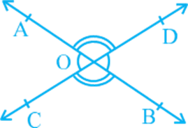
(i) ∠ AOC and ∠ BOD (ii) ∠ AOD and ∠ BOC.
We need to prove that ∠ AOC = ∠ BOD and ∠ AOD = ∠ BOC.
Now, ray OA stands on line CD.
Therefore, ∠ AOC + ∠ AOD = 180° (Linear pair axiom) (1)
Can we write ∠ AOD + ∠ BOD = 180°? Yes! (Why?) (2)
From (1) and (2), we can write
∠ AOC + ∠ AOD = ∠ AOD + ∠ BOD
This implies that ∠ AOC = ∠ BOD (Refer Section 5.2, Axiom 3)
Similarly, it can be proved that ∠AOD = ∠BOC
Now, let us do some examples based on Linear Pair Axiom and Theorem 6.1.
Parallel Lines and a Transversal
- Books Name
- Kaysons Academy Maths Foundation Book
- Publication
- Kaysons Publication
- Course
- JEE
- Subject
- Maths
Parallel Lines and a Transversal
Recall that a line which intersects two or more lines at distinct points is called a transversal (see Fig. 6.18). Line l intersects lines m and n at points P and Q respectively. Therefore, line l is a transversal for lines m and n. Observe that four angles are formed at each of the points P and Q.
Let us name these angles as ∠ 1, ∠ 2, . . ., ∠8 as shown in Fig. 6.18..
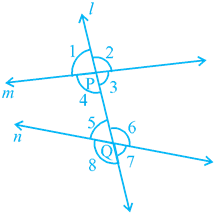
∠ 1, ∠ 2, ∠ 7 and ∠ 8 are called exterior angles, while ∠ 3, ∠ 4, ∠ 5 and ∠ 6 are called interior angles.
Recall that in the earlier classes, you have named some pairs of angles formed when a transversal intersects two lines. These are as follows:
(a) Corresponding angles:
(i) ∠ 1 and ∠ 5 (ii) ∠ 2 and ∠ 6
(b) Alternate interior angles:
(i) ∠ 4 and ∠ 6 (ii) ∠ 3 and ∠ 5
(c) Alternate exterior angles:
(i) ∠ 1 and ∠ 7 (ii) ∠ 2 and ∠ 8
(d) Interior angles on the same side of the transversal:
(i) ∠ 4 and ∠ 5 (ii) ∠ 3 and ∠ 6
Interior angles on the same side of the transversal are also referred to as consecutive interior angles or allied angles or co-interior angles. Further, many a times, we simply use the words alternate angles for alternate interior angles.
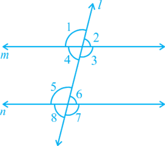
Now, let us find out the relation between the angles in these pairs when line m is parallel to line n. You know that the ruled lines of your notebook are parallel to each other. So, with ruler and pencil, draw two parallel lines along any two of these lines and a transversal to intersect them as shown in Fig. 6.19.
Now, measure any pair of corresponding angles and find out the relation between them. You may find that : ∠1 = ∠5, ∠2 = ∠6, ∠4 = ∠8 and ∠3 = ∠7. From this, you may conclude the following axiom.
Axiom 6.3: If a transversal intersects two parallel lines, then each pair of corresponding angles is equal.
Axiom 6.3 is also referred to as the corresponding angles axiom . Now, let us discuss the converse of this axiom which is as follows:
If a transversal intersects two lines such that a pair of corresponding angles is equal, then the two lines are parallel.
Does this statement hold true? It can be verified as follows: Draw a line AD and mark points B and C on it. At B and C, construct ∠ ABQ and ∠ BCS equal to each other as shown in Fig. 6.20 (i).
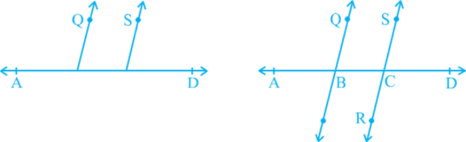
Produce QB and SC on the other side of AD to form two lines PQ and RS [see Fig. 6.20 (ii)]. You may observe that the two lines do not intersect each other. You may also draw common perpendiculars to the two lines PQ and RS at different points and measure their lengths. You will find it the same everywhere. So, you may conclude that the lines are parallel. Therefore, the converse of corresponding angles axiom is also true. So, we have the following axiom:
Axiom 6.4: If a transversal intersects two lines such that a pair of corresponding angles is equal, then the two lines are parallel to each other.
Can we use corresponding angles axiom to find out the relation between the alternate interior angles when a transversal intersects two parallel lines? In Fig. 6.21, transversal PS intersects parallel lines AB and CD at points Q and R respectively.
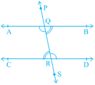
Is ∠ BQR = ∠ QRC and ∠ AQR = ∠ QRD? You know that ∠ PQA = ∠ QRC (1)
(Corresponding angles axiom)
Is ∠ PQA = ∠ BQR? Yes! (Why?) (2)
So, from (1) and (2), you may conclude that
∠ BQR = ∠ QRC.
Similarly, ∠ AQR = ∠ QRD.
This result can be stated as a theorem given below:
Theorem: If a transversal intersects two parallel lines, then each pair of alternate interior angles is equal.
Now, using the converse of the corresponding angles axiom, can we show the two lines parallel if a pair of alternate interior angles is equal? In Fig. 6.22, the transversal PS intersects lines AB and CD at points Q and R respectively such that
∠ BQR = ∠ QRC.
Is AB || CD?
∠ BQR = ∠ PQA (Why?) (1)
But, ∠ BQR = ∠ QRC (Given) (2)
So, from (1) and (2), you may conclude that
∠ PQA = ∠ QRC
But they are corresponding angles.
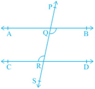
So, AB || CD (Converse of corresponding angles axiom)
This result can be stated as a theorem given below:
Theorem 6.3: If a transversal intersects two lines such that a pair of alternate interior angles is equal, then the two lines are parallel.
In a similar way, you can obtain the following two theorems related to interior angles on the same side of the transversal.
Theorem 6.4: If a transversal intersects two parallel lines, then each pair of interior angles on the same side of the transversal is supplementary.
Theorem 6.5: If a transversal intersects two lines such that a pair of interior angles on the same side of the transversal is supplementary, then the two lines are parallel.
You may recall that you have verified all the above axioms and theorems in earlier classes through activities. You may repeat those activities here also.
Lines Parallel to the Same Line
If two lines are parallel to the same line, will they be parallel to each other? Let us check it. See Fig. 6.23 in which line m || line l and line n || line l.
Let us draw a line t transversal for the lines, l, m and n. It is given that line m || line l and line n || line l.
Therefore, ∠ 1 = ∠ 2 and ∠ 1 = ∠ 3
(Corresponding angles axiom)
So, ∠ 2 = ∠ 3 (Why?)
But ∠ 2 and ∠ 3 are corresponding angles and they are equal.
Therefore, you can say that
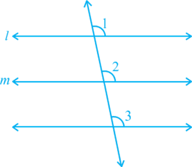
Line m || Line n
(Converse of corresponding angles axiom)
This result can be stated in the form of the following theorem:
Theorem 6.6: Lines which are parallel to the same line are parallel to each other.
Note: The property above can be extended to more than two lines also. Now, let us solve some examples related to parallel lines.
Angle Sum Property of a Triangle
In the earlier classes, you have studied through activities that the sum of all the angles of a triangle is 180°. We can prove this statement using the axioms and theorems related to parallel lines.
Theorem 6.7: The sum of the angles of a triangle is 180º.
Proof: Let us see what is given in the statement above, that is, the hypothesis and what we need to prove. We are given a triangle PQR and ∠ 1, ∠ 2 and ∠ 3 are the angles of Δ PQR (see Fig.)
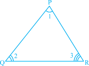
We need to prove that ∠ 1 + ∠ 2 + ∠ 3 = 180°. Let us draw a line XPY parallel to QR through the opposite vertex P, as shown in Fig. 6.35, so that we can use the properties related to parallel lines.
Now, XPY is a line.
Therefore, ∠ 4 + ∠ 1 + ∠ 5 = 180° (1)
But XPY || QR and PQ, PR are transversal.
So, ∠ 4 = ∠ 2 and ∠ 5 = ∠ 3
(Pairs of alternate angles)
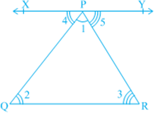
Substituting ∠ 4 and ∠ 5 in (1), we get
∠ 2 + ∠ 1 + ∠ 3 = 180°
That is, ∠ 1 + ∠ 2 + ∠ 3 = 180°
Recall that you have studied about the formation of an exterior angle of a triangle in the earlier classes (see Fig. 6.36). Side QR is produced to point S, ∠ PRS is called an exterior angle of ΔPQR.
Is ∠ 3 + ∠ 4 = 180°? (Why?) (1)
Also, see that
∠ 1 + ∠ 2 + ∠ 3 = 180° (Why?) (2)
From (1) and (2), you can see that
∠ 4 = ∠ 1 + ∠ 2.
This result can be stated in the form of a theorem as given below:
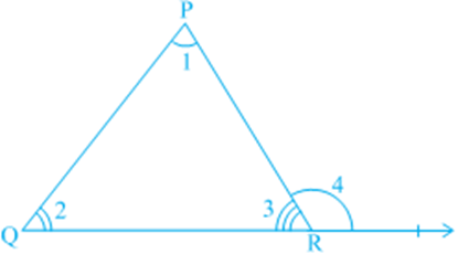
Theorem: If a side of a triangle is produced, then the exterior angle so formed is equal to the sum of the two interior opposite angles.
It is obvious from the above theorem that an exterior angle of a triangle is greater than either of its interior apposite angles.
Now, let us take some examples based on the above theorems.
Introduction
- Books Name
- Kaysons Academy Maths Foundation Book
- Publication
- Kaysons Publication
- Course
- JEE
- Subject
- Maths
Chapter -13
PROBABILITY
Introduction
In everyday life, we come across statement such as
- It will probably rain today.
- I doubt that he will pass the test.
- Most probably. Kavita will stand first in the annual examination.
- Chances are high that the prices of diesel will go up.
- There is a 50 – 50 chance of India winning a toss in today’s match.
The word ‘probably’, ‘doubt’, ‘most probably’, ‘chance’, etc., used in the statement above involve an element of uncertainty. For example, in (1), ‘probably rain’ will mean it may not rain today. We are predicting rain today based on our past experience when it rained under similar conditions. Similar predictions are also made in other cases listed in (2) to (5).
The uncertainty of ‘probably’ etc can be measured numerically by means of ‘probability’ in many cases.
Though probability started with gambling, it has been used extensively in the fields of physical Sciences, Commerce, Biological Sciences, Medical Sciences, Weather Forecasting, etc.
Probability – an Experimental Approach
In earlier classes, you have had a glimpse of probability when you performed experiments like tossing of coins, throwing of dice, etc,. and observed their outcomes. You will now learn to measure the chance of occurrence of a particular outcome in an experiment.
Write down the value of the following fractions:
![]()
And
![]()
Toss the coin twenty times and in the same way record your observations as above. Again find the values of the fractions given above for this collection of observations.
Repeat the same experiment by increasing the number of tosses and record the number of heads and tails. Then find the values of the corresponding fractions.
You will find that as the number of tosses gets larger, the values of the fractions come closer to 0.5. To record what happens in more tosses, the following group activity can also be performed:
Find the values of the following fractions:
![]()
![]()
![]()
(ii) Now throw the die 40 times, record the observations and calculate the fractions as done in (i).
As the number of throws of the die increases, you will find that the value of each fraction calculated in (1) and (2) comes closer and closer to 1/6.
To see this, you could perform a group activity, as done in Activity 2. Divide the student in your class, into small groups. One student in each group should throw a die ten times. Observations should be noted and cumulative fractions should be calculated.
The values of the fractions for the number 1 can be recorded in Table. This table can be extended to write down fractions for the other numbers also or other tables of the same kind can be created for the other numbers.
Write down the fractions:
![]()
![]()
![]()
Calculate the values of these fractions.
Now, increases the number of tosses (as in Activity 2). You will find that the more the number of tosses, the closer are the values of A, B and C to 0.25, 0.5 and 0.25, respectively.
In Activity 1, each toss of a coin is called a trial. Similarly in Activity 3, each throw of a die is a trial, and each simultaneous toss of two coin in Activity 4 is also a trial.
So, a trial is an action which results in one or several outcomes. The possible outcomes in Activity 1 were Head and Tail; whereas in Activity 1 where Head and Tail; whereas in Activity 3, the possible outcomes were 1, 2, 3, 4, 5 and 6.
In Activity 1, the getting of a head in a particular throw is an event with outcome ‘head’. Similarly, getting a tail is an event with outcome ‘tail’. In Activity 2, the getting of a particular number, say 1, is and event with outcome 1.
If your experiment was to throw the die for getting an even number, then the event would consist of three outcomes, namely, 2, 4 and 6.
So, an event for an experiment is the collection of some outcomes of the experiment. In class X, you will study a more formula definition of an event.
So, can you now tell what the events are in Activity 4?
With this background, let us now see what probability is. Based on what we directly observe as the outcomes of our trials, we find the experimental or empirical probability.
Let n be the total number of trials. The empirical probability P (E) of an event E happening, is given by
![]()
In this chapter, we shall be finding the empirical probability, though we will write ‘probability’ for convenience,
Let us consider some examples.
To start with let us go back to Activity 2, and Table 15.2. in Column (4) of this table, what is the fraction that you calculate? Nothing, but it is the empirical probability of getting a head. Note that this probability kept changing depending on the number of trials and the number of heads obtained in these trials. Similarly, the empirical probability of getting a tail is obtained in Column (5) of Table. This is 12/15 to start with, then it is 2/3, then 28/45, and so on.
So, the empirical probability depends on the number of trials undertaken, and the number of times the outcomes you are looking for coming up in these trials.
Activity
Before going further, look at the tables you drew up while doing Activity 3. Find the probabilities of getting a 3 when throwing a die a certain number of times. Also, show how it changes as the number of trials increases.
Now, let us consider some other examples.
Angle Sum Property of a Quadrilateral
- Books Name
- Kaysons Academy Maths Foundation Book
- Publication
- Kaysons Publication
- Course
- JEE
- Subject
- Maths
Chapter -8
Quadrilaterals
A quadrilateral has four sides, four angles and four vertices [see Fig. (i)].
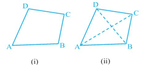
In quadrilateral ABCD, AB, BC, CD and DA are the four sides; A, B, C and D are the four vertices and ∠ A, ∠ B, ∠ C and ∠ D are the four angles formed at the vertices.
Now join the opposite vertices A to C and B to D [see Fig (ii)]. AC and BD are the two diagonals of the quadrilateral ABCD.
In this chapter, we will study more about different types of quadrilaterals, their properties and especially those of parallelograms.You may wonder why should we study about quadrilaterals (or parallelograms) Look around you and you will find so many objects which are of the shape of a quadrilateral - the floor, walls, ceiling, windows of your classroom, the blackboard, each face of the duster, each page of your book, the top of your study table etc. Some of these are given below (see Fig).
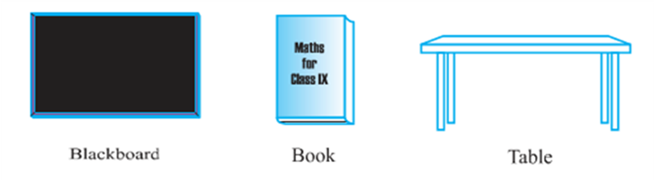
Although most of the objects we see around are of the shape of special quadrilateral called rectangle, we shall study more about quadrilaterals and especially parallelograms because a rectangle is also a parallelogram and all properties of a parallelogram are true for a rectangular as well.
Angle Sum Property of a Quadrilateral
Let us now recall the angle sum property of a quadrilateral.
The sum of the angles of a quadrilateral is 360º. This can be verified by drawing a diagonal and dividing the quadrilateral into two triangles.
Let ABCD be a quadrilateral and AC be a diagonal (see Fig).
What is the sum of angles in Δ ADC?
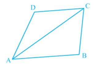
You know that
![]()
Similarly, in
![]()
Adding (1) and (2), we get
![]()
![]()
![]()
i.e., the sum of the angles of a quadrilateral is 360o.
Look at the different quadrilaterals drawn below
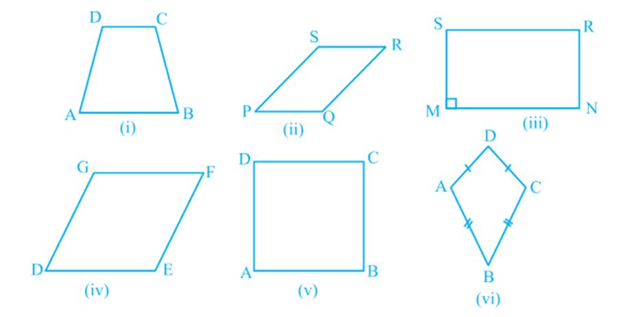
Observe that:
One pair of opposite sides of quadrilateral ABCD is Fig. (i) namely, AB and CD parallel. You know that it is called a trapezium.
Both pairs of opposite sides of quadrilaterals given in Fig. (ii), (iii), (iv) and (v) are parallel. Recall that such quadrilaterals are called parallelograms.
So, quadrilateral PQRS of Fig. (ii) is a parallelogram.
Properties of a Parallelogram
- Books Name
- Kaysons Academy Maths Foundation Book
- Publication
- Kaysons Publication
- Course
- JEE
- Subject
- Maths
Properties of a Parallelogram
Let us perform an activity.
Cut out a parallelogram from a sheet of paper and cut it along a diagonal (see Fig). You obtain two triangles. What can you say about these triangles?
Place one triangle over the other. Turn one around, if necessary. What do you observe?
Observe that the two triangles are congruent to each other.
Repeat this activity with some more parallelograms. Each time you will observe that each diagonal divides the parallelogram into two congruent triangles.
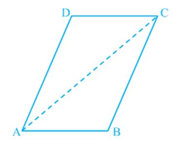
Another Condition for a Quadrilateral to be a Parallelogram
You have studied many properties of a parallelogram in this chapter and you have also verified that if in a quadrilateral any one of those properties is satisfied, then it becomes a parallelogram.
We now study yet another condition which is the least required condition for a quadrilateral to be a parallelogram.
It is stated in the form of a theorem as given below:
The Mid –point Theorem
You have studied many properties of a triangle as well as a quadrilateral. Now let us study yet another result which is related to the mid-point of sides of a triangle. Perform the following activity.
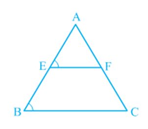
Draw a triangle and mark the mid-points E and F of two sides of the triangle. Join the points E and F (see Fig).
Measure EF and BC. Measure ∠AEF and ∠ABC.
What do you observe? You will find that:
![]()
So, EF || BC
Repeat this activity with some more triangles.
So, you arrive at the following theorem:
Collection of Data
- Books Name
- Kaysons Academy Maths Foundation Book
- Publication
- Kaysons Publication
- Course
- JEE
- Subject
- Maths
Chapter -12
STATISTICS
Collection of Data
Let us begin with an exercise on gathering data by performing the following activity.
Activity 1: Divide the students of your class into four groups. Allot each group the work of collecting one of the following kinds of data:
(i) Heights of 20 students of your class.
(ii) Number of absentees in each day in your class for a month.
(iii) Number of members in the families of your classmates.
(iv) Heights of 15 plants in or around your school.
Let us move to the results students have gathered. How did they collect their data in each group?
(i) Did they collect the information from each and every student, house or person concerned for obtaining the information?
(ii) Did they get the information from some source like available school records?
In the first case, when the information was collected by the investigator herself or himself with a definite objective in her or his mind, the data obtained is called primary data.
In the second case, when the information was gathered from a source which already had the information stored, the data obtained is called secondary data. Such data, which has been collected by someone else in another context, needs to be used with great care ensuring that the source is reliable.
Presentation of Data
As soon as the work related to collection of data is over, the investigator has to find out ways to present them in a form which is meaningful, easily understood and gives its main features at a glance. Let us now recall the various ways of presenting the data through some examples.
Example 1: Consider the marks obtained by 10 students in a mathematics test as given below:
25 36 42 55 60 62 73 75 78 95
Now, we can clearly see that the lowest marks are 25 and the highest marks are 95. The difference of the highest and the lowest values in the data is called the range of the data. So, the range in this case is 95 – 25 = 70.
Presentation of data in ascending or descending order can be quite time consuming, particularly when the number of observations in an experiment is large, as in the case of the next example.
Example 2: Consider the marks obtained (out of 100 marks) by 30 students of Class
IX of a school:
10 20 36 92 95 40 50 56 60 70
92 88 80 70 72 70 36 40 36 40
92 40 50 50 56 60 70 60 60 88

Recall that the number of students who have obtained a certain number of marks is called the frequency of those marks. For instance, 4 students got 70 marks. So the frequency of 70 marks is 4. To make the data more easily understandable, we write it in a table, as given below:
Table is called an ungrouped frequency distribution table, or simply a frequency distribution table. Note that you can use also tally marks in preparing these tables, as in the next example.
Graphical Representation of Data
The representation of data by tables has already been discussed. Now let us turn our attention to another representation of data, i.e., the graphical representation. It is well said that one picture is better than a thousand words. Usually comparisons among the individual items are best shown by means of graphs. The representation then becomes easier to understand than the actual data. We shall study the following graphical representations in this section.
(A) Bar graphs
(B) Histograms of uniform width, and of varying widths
(C) Frequency polygons
(A) Bar Graphs
In earlier classes, you have already studied and constructed bar graphs. Here we shall discuss them through a more formal approach. Recall that a bar graph is a pictorial representation of data in which usually bars of uniform width are drawn with equal spacing between them on one axis (say, the x-axis), depicting the variable. The values of the variable are shown on the other axis (say, the y-axis) and the heights of the bars depend on the values of the variable.
(B) Histogram
This is a form of representation like the bar graph, but it is used for continuous class intervals. For instance, consider the frequency distribution Table 14.6, representing the weights of 36 students of a class:

Let us represent the data given above graphically as follows:
(i) We represent the weights on the horizontal axis on a suitable scale. We can choose the scale as 1 cm = 5 kg. Also, since the first class interval is starting from 30.5 and not zero, we show it on the graph by marking a kink or a break on the axis.
(ii) We represent the number of students (frequency) on the vertical axis on a suitable scale. Since the maximum frequency is 15, we need to choose the scale to accomodate this maximum frequency.
(iii) We now draw rectangles (or rectangular bars) of width equal to the class-size and lengths according to the frequencies of the corresponding class intervals. For example, the rectangle for the class interval 30.5 - 35.5 will be of width 1 cm and length 4.5 cm.
(iv) In this way, we obtain the graph as shown in Fig.
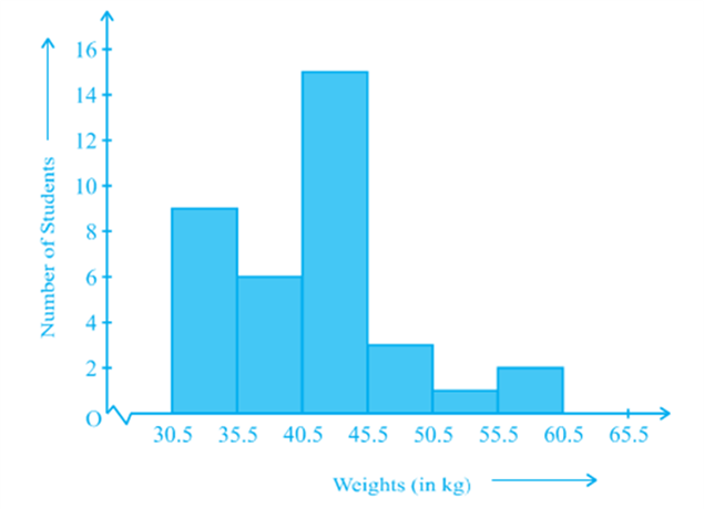
Observe that since there are no gaps in between consecutive rectangles, the resultant graph appears like a solid figure. This is called a histogram, which is a graphical representation of a grouped frequency distribution with continuous classes. Also, unlike a bar graph, the width of the bar plays a significant role in its construction.
Here, in fact, areas of the rectangles erected are proportional to the corresponding frequencies. However, since the widths of the rectangles are all equal, the lengths of the rectangles are proportional to the frequencies. That is why, we draw the lengths according to (iii) above.
(C) Frequency Polygon
There is yet another visual way of representing quantitative data and its frequencies. This is a polygon. To see what we mean, consider the histogram represented by Fig. Let us join the mid-points of the upper sides of the adjacent rectangles of this histogram by means of line segments. Let us call these mid-points B, C, D, E, F and G. When joined by line segments, we obtain the figure BCDEFG (see Fig.) To complete the polygon, we assume that there is a class interval with frequency zero before 30.5 - 35.5, and one after
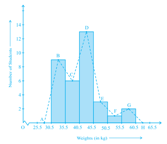
55.5 - 60.5, and their mid-points are A and H, respectively. ABCDEFGH is the frequency polygon corresponding to the data shown in Fig. We have shown this in Fig.
Although, there exists no class preceding the lowest class and no class succeeding the highest class, addition of the two class intervals with zero frequency enables us to make the area of the frequency polygon the same as the area of the histogram. Why is this so? (Hint: Use the properties of congruent triangles.)
Now, the question arises: how do we complete the polygon when there is no class preceding the first class? Let us consider such a situation.
Measures of Central Tendency
- Books Name
- Kaysons Academy Maths Foundation Book
- Publication
- Kaysons Publication
- Course
- JEE
- Subject
- Maths
Measures of Central Tendency
Earlier in this chapter, we represented the data in various forms through frequency distribution tables, bar graphs, histograms and frequency polygons. Now, the question arises if we always need to study all the data to ‘make sense’ of it, or if we can make out some important features of it by considering only certain representatives of the data. This is possible, by using measures of central tendency or averages.
Consider a situation when two students Mary and Hari received their test copies. The test had five questions, each carrying ten marks. Their scores were as follows:
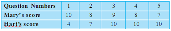
Upon getting the test copies, both of them found their average scores as follows:
![]()
![]()
Since Mary’s average score was more than Hari’s, Mary claimed to have performed better than Hari, but Hari did not agree. He arranged both their scores in ascending order and found out the middle score as given below:
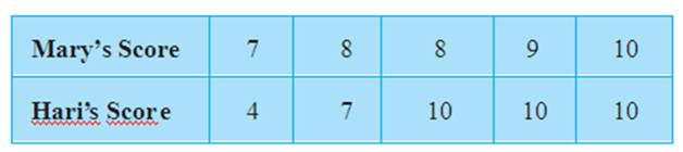
Hari said that since his middle-most score was 10, which was higher than Mary’s middle-most score, that is 8, his performance should be rated better.
But Mary was not convinced. To convince Mary, Hari tried out another strategy. He said he had scored 10 marks more often (3 times) as compared to Mary who scored 10 marks only once. So, his performance was better.
Now, to settle the dispute between Hari and Mary, let us see the three measures they adopted to make their point.
The average score that Mary found in the first case is the mean. The ‘middle’ score that Hari was using for his argument is the median. The most often scored mark that Hari used in his second strategy is the mode.
Now, let us first look at the mean in detail.
The mean (or average) of a number of observations is the sum of the values of all the observations divided by the total number of observations.
It is denoted by the symbol x , read as ‘x bar’.
Let us consider an example.
The median is that value of the given number of observations, which divides it into exactly two parts. So, when the data is arranged in ascending (or descending) order the median of ungrouped data is calculated as follows:
(i) When the number of observations (n) is odd, the median is the value of the ![]() observation. For example, if n = 13, the value of the
observation. For example, if n = 13, the value of the ![]() is., the 7th observation will be the median [see Fig (i)]
is., the 7th observation will be the median [see Fig (i)]
(ii) When the number of observations (n) is even, the median is the mean of the ![]() observations. For example, if n = 16, the mean of the value of the
observations. For example, if n = 16, the mean of the value of the ![]() observations, i.e., the mean of the values of the 8th and 9th observations will be the median [see Fig. (ii)].
observations, i.e., the mean of the values of the 8th and 9th observations will be the median [see Fig. (ii)].
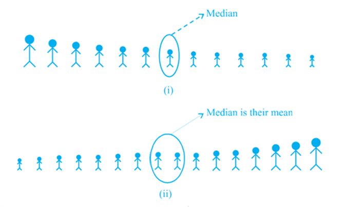
The mode is that value of the observation with occurs most frequently, i.e., an observation with the maximum frequency is called the mode.
The ready made garment and shoe industries make great use of this measure of central tendency. Using the knowledge of mode, these industries decide which size of the product should be produced in large numbers.