 Kaysons Publication
Theorem (Euclid’s Division Lemma)
- Books Name
- Kaysons Academy Maths Foundation Book
- Publication
- Kaysons Publication
- Course
- JEE
- Subject
- Maths
Chapter -1
Real Number
Theorem (Euclid’s Division Lemma): Given positive integers a and b, there exist unique integers q and r satisfying a = bq + r, 0 ≤ r < b.
To obtain the HCF of two positive integers, say c and d, with c > d, follow the steps below:
Step 1: Apply Euclid’s division lemma, to c and d. So, we find whole numbers, q and r such that c = dq + r, 0 ≤ r < d.
Step 2: If r = 0, d is the HCF of c and d. If r ≠ 0, apply the division lemma to d and r.
Step 3: Continue the process till the remainder is zero. The divisor at this stage will be the required HCF.
This algorithm works because HCF (c, d) = HCF (d, r) where the symbol HCF (c, d) denotes the HCF of c and d, etc.
The Fundamental Theorem of Arithmetic
In your earlier classes, you have seen that any natural number can be written as a product of its prime factors. For instance, 2 = 2, 4 = 2 × 2, 253 = 11 × 23, and so on. Now, let us try and look at natural numbers from the other direction. That is, can any natural number be obtained by multiplying prime numbers? Let us see.
Take any collection of prime numbers, say 2, 3, 7, 11 and 23. If we multiply some or all of these numbers, allowing them to repeat as many times as we wish, we can produce a large collection of positive integers (In fact, infinitely many).
Let us list a few:
7 × 11 × 23 = 1771 3 × 7 × 11 × 23 = 5313
2 × 3 × 7 × 11 × 23 = 10626 23 × 3 × 73 = 8232
22 × 3 × 7 × 11 × 23 = 21252
and so on.
Theorem (Fundamental Theorem of Arithmetic): Every composite number can be expressed (factorised) as a product of primes, and this factorization is unique, apart from the order in which the prime factors occur.
The prime factorisation of a natural number is unique, except for the order of its factors.
In general, given a composite number x, we factorise it as x = p1p2 ... pn, where p1, p2,..., pn are primes and written in ascending order, i.e., p1 ≤ p2 ≤. . . ≤ pn. If we combine the same primes, we will get powers of primes. For example,
32760 = 2 × 2 × 2 × 3 × 3 × 5 × 7 × 13 = 23 × 32 × 5 × 7 × 13
Revisiting Irrational Numbers
- Books Name
- Kaysons Academy Maths Foundation Book
- Publication
- Kaysons Publication
- Course
- JEE
- Subject
- Maths
Revisiting Irrational Numbers
In Class IX, you were introduced to irrational numbers and many of their properties. You studied about their existence and how the rationals and the irrationals together made up the real numbers. You even studied how to locate irrationals on the number line. However, we did not prove that they were irrationals. In this section, we will prove that ![]() and, in general,
and, in general, ![]() is irrational, where p is a prime. One of the theorems, we use in our proof, is the Fundamental Theorem of Arithmetic.
is irrational, where p is a prime. One of the theorems, we use in our proof, is the Fundamental Theorem of Arithmetic.
Recall, a number‘s’ is called irrational if it cannot be written in the form![]() where p and q are integers and q ≠ 0. Some examples of irrational numbers, with which you are already familiar, are:
where p and q are integers and q ≠ 0. Some examples of irrational numbers, with which you are already familiar, are:
![]()
Before we prove that 2 is irrational, we need the following theorem, whose proof is based on the Fundamental Theorem of Arithmetic.
Revisiting Rational Numbers and Their Decimal Expansions
In Class IX, you studied that rational numbers have either a terminating decimal expansion or a non-terminating repeating decimal expansion. In this section, we are going to consider a rational number, say
![]() and explore exactly when the decimal expansion of
and explore exactly when the decimal expansion of ![]() is terminating and when it is non-terminating and when it is non-terminating repeating (or recurring). We do so by considering several examples.
is terminating and when it is non-terminating and when it is non-terminating repeating (or recurring). We do so by considering several examples.
Let us consider the following rational numbers:
(i) 0.375 (ii) 0.104 (iii) 0.0875 (iv) 23.3408.
![]()
![]()
As one would expect, they can all be expressed as rational numbers whose denominators are powers of 10. Let us try and cancel the common factors between the numerator an denominator and see what we get:
![]()
![]()
Theorem: Let x be a rational number whose decimal expansion terminates.
Then x can be expressed in the form
![]() where p and q are coprime, and the prime factorization of q is of the form 2n5m, where n, m are non-negative integers.
where p and q are coprime, and the prime factorization of q is of the form 2n5m, where n, m are non-negative integers.
Theorem: Let ![]() be a rational number, such that the prime factorization of q is of the form 2n5m, where n, m are non-negative integers. Then x has a decimal expansion which terminates.
be a rational number, such that the prime factorization of q is of the form 2n5m, where n, m are non-negative integers. Then x has a decimal expansion which terminates.
The Polynomial p(x).
- Books Name
- Kaysons Academy Maths Foundation Book
- Publication
- Kaysons Publication
- Course
- JEE
- Subject
- Maths
Chapter -2
POLYNOMISALS
The Polynomial p(x)
For example, 4x + 2 is a polynomial in the variable x of degree 1, 2y2 – 2y + 4 is a polynomial in the variable y of degree
![]() is a polynomial in the variable x of degree 3 and
is a polynomial in the variable x of degree 3 and![]() is a polynomial in the variable u of degree 6. Expressions like
is a polynomial in the variable u of degree 6. Expressions like ![]() , are not polynomials.
, are not polynomials.
A polynomial of degree 1 is called a linear polynomial. For example, ![]() are all linear polynomials. Polynomials such as 2x + 5 – x2, x3 + 1, etc., are not linear polynomials.
are all linear polynomials. Polynomials such as 2x + 5 – x2, x3 + 1, etc., are not linear polynomials.
A polynomial of degree 2 is called a quadratic polynomial. The name ‘quadratic’ has been derived from the word ‘quadratie’ which means ‘square’.
![]() are some examples of quadratic polynomials (whose coefficient are real numbers). More generally, any quadratic polynomial in x is of the form ax2 + bx + c, where a, b, c are real numbers and
are some examples of quadratic polynomials (whose coefficient are real numbers). More generally, any quadratic polynomial in x is of the form ax2 + bx + c, where a, b, c are real numbers and ![]() In fact, the most general form of a cubic polynomial is ax3 + bx2 + cx + d.
In fact, the most general form of a cubic polynomial is ax3 + bx2 + cx + d.
Where, a, b, c, d are real numbers and
Now consider the polynomial p(x) = x2 – 3x – 4. Then, putting x = 2 in the polynomial, we get p(2) = 22 – 3 × 2 – 4 = – 6. The value ‘– 6’, obtained by replacing x by 2 in x2 – 3x – 4, is the value of x2 – 3x – 4 at x = 2. Similarly, p(0) is the value of p(x) at x = 0, which is – 4.
If p(x) is a polynomial in x, and if k is any real number, then the value obtained by replacing x by k in p(x), is called the value of p(x) at x = k, and is denoted by p(k). What is the value of p(x) = x2 –3x – 4 at x = –1? We have:
p(–1) = (–1)2 –{3 × (–1)} – 4 = 0
Also, note that p(4) = 42 – (3 × 4) – 4 = 0.
As p(–1) = 0 and p(4) = 0, –1 and 4 are called the zeroes of the quadratic polynomial x2 – 3x – 4. More generally, a real number k is said to be a zero of a polynomial p(x), if p(k) = 0.
You have already studied in Class IX, how to find the zeroes of a linear polynomial. For example, if k is a zero of p(x) = 2x + 3, then p(k) = 0 gives us 2k + 3 = 0, i.e.,
![]()
In general, if k is a zero of p(x) = ax + b, then p(k) = ak + b = 0, i.e., ![]()
So, the zero of the linear polynomial ax + b is ![]()
Thus, the zero of a linear polynomial is related to its coefficients. Does this happen in the case of other polynomials too? For example, are the zeroes of a quadratic polynomial also related to its coefficients?
In this chapter, we will try to answer these questions. We will also study the division algorithm for polynomials.
Geometrical Meaning of the Zeroes of a Polynomial
You know that a real number k is a zero of the polynomial p(x) if p(k) = 0. But why are the zeroes of a polynomial so important? To answer this, first we will see the geometrical representations of linear and quadratic polynomials and the geometrical meaning of their zeroes.
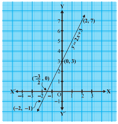
Consider first a linear polynomial ax + b, a ≠ 0. You have studied in Class IX that the graph of y = ax + b is a straight line. For example, the graph of y = 2x + 3 is a straight line passing through the points (– 2, –1) and (2, 7).
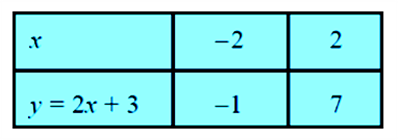
From Fig. 2.1, you can see that the graph of y = 2x + 3 intersects the x -axis mid-way between x = –1 and x = – 2, that is, at the point ![]()
You also know that the zero of 2x + 3 is ![]() Thus, the zero of the polynomial 2x + 3 is the x-coordinate of the point where the graph of y = 2x + 3 intersects the x-axis. In general, for a linear polynomial
Thus, the zero of the polynomial 2x + 3 is the x-coordinate of the point where the graph of y = 2x + 3 intersects the x-axis. In general, for a linear polynomial ![]() Therefore, the linear polynomial
Therefore, the linear polynomial
Relationship between Zeroes and Coefficients of a Polynomial
- Books Name
- Kaysons Academy Maths Foundation Book
- Publication
- Kaysons Publication
- Course
- JEE
- Subject
- Maths
Relationship between Zeroes and Coefficients of a Polynomial
You have already seen that zero of a linear polynomial ax + b is
![]() We will now try to answer the question raised in Section 2.1 regarding the relationship between zeroes and coefficients of a quadratic polynomial. For this, let us take a quadratic polynomial, say p(x) = 2x2 – 8x + 6. In Class IX, you have learnt how to factorise quadratic polynomials by splitting the middle term. So, here we need to split the middle term ‘– 8x’ as a sum of two terms, whose product is 6 × 2x2 = 12x2. So, we write
We will now try to answer the question raised in Section 2.1 regarding the relationship between zeroes and coefficients of a quadratic polynomial. For this, let us take a quadratic polynomial, say p(x) = 2x2 – 8x + 6. In Class IX, you have learnt how to factorise quadratic polynomials by splitting the middle term. So, here we need to split the middle term ‘– 8x’ as a sum of two terms, whose product is 6 × 2x2 = 12x2. So, we write
2x2 – 8x + 6 = 2x2 – 6x – 2x + 6 = 2x(x – 3) – 2(x – 3)
= (2x – 2)(x – 3) = 2(x – 1)(x – 3)
So, the value of p(x) = 2x2 – 8x + 6 is zero when x – 1 = 0 or x – 3 = 0, i.e., when x = 1 or x = 3. So, the zeroes of 2x2 – 8x + 6 are 1 and 3. Observe that:
![]()
![]()
Let us take one more quadratic polynomial, say, p(x) = 3x2 + 5x – 2. By the method of splitting the middle term,
![]()
![]()
Hence, the value of 3x2 + 5x – 2 is zero when either 3x – 1 = 0 or x + 2 = 0, i.e.,
![]() Observe that:
Observe that:
![]()
![]()
In general, if α* and β* are the zeroes of the quadratic polynomial p(x) = ax2 + bx + c,
![]() are the factors of p(x). Therefore,
are the factors of p(x). Therefore,
![]() where k is a constant
where k is a constant
![]()
![]()
Comparing the coefficients of x2, x and constant terms on both the sides, we get
![]()
![]()
![]()
Division algorithm for Polynomials
You know that a cubic polynomial has at most three zeroes. However, if you are given only one zero, can you find the other two? For this, let us consider the cubic polynomial
![]() If we tell you that one of its zeroes is 1, then you know that x – 1 is a factor of x3 – 3x2 – x + 3. So, you can divide x3 – 3x2 – x + 3 by x – 1, as you have learnt in Class IX, to get quotient x2 – 2x – 3.
If we tell you that one of its zeroes is 1, then you know that x – 1 is a factor of x3 – 3x2 – x + 3. So, you can divide x3 – 3x2 – x + 3 by x – 1, as you have learnt in Class IX, to get quotient x2 – 2x – 3.
Next, you could get the factors of x2 – 2x – 3, by splitting the middle term, as (x + 1) (x – 3). This word give you
![]()
![]()
So, all the three zeroes of the cubic polynomial are now known to you as 1, – 1, 3.
Let us discuss the method of dividing one polynomial by another in some detail.
Before noting the steps formally.
![]() then we can find polynomials q(x) and r(x) such that
then we can find polynomials q(x) and r(x) such that
![]()
Where r(x) = 0 or degree of r (x) < degree of g(x).
Pair of Linear Equations in Two Variables
- Books Name
- Kaysons Academy Maths Foundation Book
- Publication
- Kaysons Publication
- Course
- JEE
- Subject
- Maths
Chapter -3
Pair of Linear Equations in Two Variables
Pair of Linear Equations in Two Variables
Recall, from Class IX, that the following are examples of linear equations in two variables:
2x + 3y = 5
x – 2y – 3 = 0
and x – 0y = 2, i.e., x = 2s
You also know that an equation which can be put in the form ax + by + c = 0, where a, b and c are real numbers, and a and b are not both zero, is called a linear equation in two variables x and y. (We often denote the condition a and b are not both zero by a2 + b2 ≠ 0). You have also studied that a solution of such an equation is a pair of values, one for x and the other for y, which makes the two sides of the equation equal.
For example, let us substitute x = 1 and y = 1 in the left hand side (LHS) of the equation 2x + 3y = 5. Then
LHS = 2(1) + 3(1) = 2 + 3 = 5,
which is equal to the right hand side (RHS) of the equation. Therefore, x = 1 and y = 1 is a solution of the equation 2x + 3y = 5. Now let us substitute x = 1 and y = 7 in the equation 2x + 3y = 5. Then,
LHS = 2(1) + 3(7) = 2 + 21 = 23 which is not equal to the RHS.
Therefore, x = 1 and y = 7 is not a solution of the equation.
Geometrically, what does this mean? It means that the point (1, 1) lies on the line representing the equation 2x + 3y = 5, and the point (1, 7) does not lie on it. So, every solution of the equation is a point on the line representing it.
In fact, this is true for any linear equation, that is, each solution (x, y) of a linear equation in two variables, ax + by + c = 0, corresponds to a point on the line representing the equation, and vice versa.
Now, consider Equations (1) and (2) given above. These equations, taken together, represent the information we have about Akhila at the fair.
These two linear equations are in the same two variables x and y. Equations like these are called a pair of linear equations in two variables.
Graphical Method of Solution of a Pair of Linear Equations
In the previous section, you have seen how we can graphically represent a pair of linear equations as two lines. You have also seen that the lines may intersect, or may be parallel, or may coincide. Can we solve them in each case? And if so, how? We shall try and answer these questions from the geometrical point of view in this section.
Let us look at the earlier examples one by one.
l In the situation of Example 1, find out how many rides on the Giant Wheel Akhila had, and how many times she played Hoopla.
In Fig. 3.2, you noted that the equations representing the situation are geometrically shown by two lines intersecting at the point (4, 2). Therefore, the point (4, 2) lies on the lines represented by both the equations x – 2y = 0 and 3x + 4y = 20. And this is the only common point.
Let us verify algebraically that x = 4, y = 2 is a solution of the given pair of equations. Substituting the values of x and y in each equation, we get
4 – 2 × 2 = 0 and 3(4) + 4(2) = 20. So, we have verified that x = 4, y = 2 is a solution of both the equations. Since (4, 2) is the only common point on both the lines, there is one and only one solution for this pair of linear equations in two variables.
We can now summarise the behavior of lines representing a pair of linear equations in two variables and the existence of solutions as follows:
(i) The lines may intersect in a single point. In this case, the pair of equations has a unique solution (consistent pair of equations).
(ii) The lines may be parallel. In this case, the equations have no solution (Inconsistent pair of equations).
(iii) The lines may be coincident. In this case, the equations have infinitely many solutions [dependent (consistent) pair of equations].
Let us now go back to the pairs of linear equations formed in Examples 1, 2, and 3, and note down what kind of pair they are geometrically.
(i) x – 2y = 0 and 3x + 4y – 20 = 0 (The lines intersect)
(ii) 2x + 3y – 9 = 0 and 4x + 6y – 18 = 0 (The lines coincide)
(iii) x + 2y – 4 = 0 and 2x + 4y – 12 = 0 (The lines are parallel)
Algebraic Methods of Solving a Pair of Linear Equations
- Books Name
- Kaysons Academy Maths Foundation Book
- Publication
- Kaysons Publication
- Course
- JEE
- Subject
- Maths
Algebraic Methods of Solving a Pair of Linear Equations
In the previous section, we discussed how to solve a pair of linear equations graphically. The graphical method is not convenient in cases when the point representing the solution of the linear equations has non-integral coordinates like ![]()
![]() etc. There is every possibility of making mistakes while reading such coordinates. Is there any alternative method of finding the solution? There are several algebraic methods, which we shall now discuss.
etc. There is every possibility of making mistakes while reading such coordinates. Is there any alternative method of finding the solution? There are several algebraic methods, which we shall now discuss.
Substitution Method: We shall explain the method of substitution by taking some examples.
Example: Solve the following pair of equations by substitution method:
7x – 15y = 2 (1)
x + 2y = 3 (2)
Solution:
Step 1: We pick either of the equations and write one variable in terms of the other. Let us consider the Equation (2):
x + 2y = 3
and write it as x = 3 – 2y (3)
Step 2: Substitute the value of x in Equation (1). We get
7(3 – 2y) – 15y = 2
i.e., 21 – 14y – 15y = 2
i.e., – 29y = –19
Therefore, ![]()
Step 3: Substituting this value of y in Equation (3), we get
![]()
Therefore, the solution is ![]()
Verification: Substituting x = 29 and y = 29, you can verify that both the Equations
(1) and (2) are satisfied.
Remark: We have substituted the value of one variable by expressing it in terms of the other variable to solve the pair of linear equations. That is why the method is known as the substitution method.
Elimination Method
Now let us consider another method of eliminating (i.e., removing) one variable. This is sometimes more convenient than the substitution method. Let us see how this method works.
Cross - Multiplication Method
So far, you have learnt how to solve a pair of linear equations in two variables by graphical, substitution and elimination methods. Here, we introduce one more algebraic method to solve a pair of linear equations which for many reasons is a very useful method of solving these equations. Before we proceed further, let us consider the following situation.
Let us now see how this method works for any pair of linear equations in two variables of the form
a1x + b1y + c1 = 0 (1)
and a2x + b2y + c2 = 0 (2)
To obtain the values of x and y as shown above, we follow the following steps:
Step 1: Multiply Equation (1) by b2 and Equation (2) by b1, to get
b2a1x + b2b1y + b2c1 = 0 (3)
b1a2x + b1b2y + b1c2 = 0 (4)
Step 2: Subtracting Equation (4) from (3), we get:
(b2a1 – b1a2) x + (b2b1 – b1b2) y + (b2c1 – b1c2) = 0
i.e., (b2a1 – b1a2) x = b1c2 – b2c1
![]() (5)
(5)
Step 3: Substituting this value of x in (1) or (2), we get
![]() (6)
(6)
Now, two cases arise:
Case 1: a1b2 – a2b1 ≠ 0. In this case ![]() Then the pair of linear equations has a unique solution.
Then the pair of linear equations has a unique solution.
Case 2: a1b2 – a2b1 = 0. If we write
![]() then a1 = k a2, b1 = k b2.
then a1 = k a2, b1 = k b2.
Substituting the values of a1 and b1 in the Equation (1), we get
k(a2x + b2y) + c1 = 0. (7)
It can be observed that the Equations (7) and (2) can both be satisfied only if
c1 = k c2, i.e., ![]()
If c1 = k c2, any solution of Equation (2) will satisfy the Equation (1), and vice versa. So, if ![]() , then there are infinitely many solutions to the pair of linear equations given by (1) and (2).
, then there are infinitely many solutions to the pair of linear equations given by (1) and (2).
If c1 ≠ k c2, then any solution of Equation (1) will not satisfy Equation (2) and vice versa. Therefore the pair has no solution.
We can summarise the discussion above for the pair of linear equations given by (1) and (2) as follows:
(i) When ![]() we get a unique solution.
we get a unique solution.
(ii) When ![]() there are infinitely many solutions.
there are infinitely many solutions.
(iii) When ![]() there is no solution.
there is no solution.
Note that you can write the solution given by Equations (5) and (6) in the following form:
![]() (8)
(8)
In remembering the above result, the following diagram may be helpful to you:

The arrows between the two numbers indicate that they are to be multiplied and the second product is to be subtracted from the first.
For solving a pair of linear equations by this method, we will follow the following steps:
Step 1: Write the given equations in the form (1) and (2).
Step 2: Taking the help of the diagram above, write Equations as given in (8).
Step 3: Find x and y, provided a1b2 – a1b1 ≠ 0
Step 2 above gives you an indication of why this method is called the cross-multiplication method.
Equations Reducible to a Pair of Linear Equations in Two Variables
In this section, we shall discuss the solution of such pairs of equations which are not linear but can be reduced to linear form by making some suitable substitutions. We now explain this process through some examples.
Introduction
- Books Name
- Kaysons Academy Maths Foundation Book
- Publication
- Kaysons Publication
- Course
- JEE
- Subject
- Maths
Chapter -4
TRIANGLES
Introduction
In Class IX, you have seen that all circles with the same radii are congruent, all squares with the same side lengths are congruent and all equilateral triangles with the same side lengths are congruent.
Now consider any two (or more) circles [see Fig (i)]. Are they congruent? Since all of them do not have the same radius, they are not congruent to each other. Note that some are congruent and some are not, but all of them have the same shape. So they all are, what we call, similar. Two similar figures have the same shape but not necessarily the same size. Therefore, all circles are similar. What about two (or more) squares or two (or more) equilateral triangles [see Fig (ii) and (iii)]? As observed in the case of circles, here also all squares are similar and all equilateral triangles are similar.

From the above, we can say that all congruent figures are similar but the similar figures need not be congruent. Can a circle and a square be similar? Can a triangle and a square be similar? These questions can be answered by just looking at the figures (see Fig). Evidently these figures are not similar. (Why?)
What can you say about the two quadrilaterals ABCD and PQRS (see Fig.1)? Are they similar? These figures appear to be similar but we cannot be certain about it. Therefore, we must have some definition of similarity of figures and based on this definition some rules to decide whether the two given figures are similar or not. For this, let us look at the photographs given in Fig. 2:
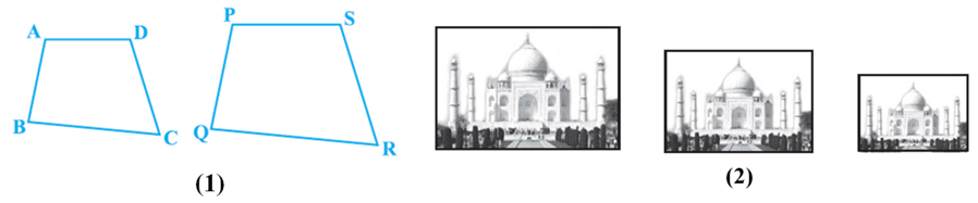
You will at once say that they are the photographs of the same monument (Taj Mahal) but are in different sizes. Would you say that the three photographs are similar? Yes, they are.
What can you say about the two photographs of the same size of the same person one at the age of 10 years and the other at the age of 40 years? Are these photographs similar? These photographs are of the same size but certainly they are not of the same shape. So, they are not similar.
What does the photographer do when she prints photographs of different sizes from the same negative? You must have heard about the stamp size, passport size and postcard size photographs. She generally takes a photograph on a small size film, say of 35mm size and then enlarges it into a bigger size, say 45mm (or 55mm). Thus, if we consider any line segment in the smaller photograph (figure), its corresponding line segment in the bigger photograph (figure) will be ![]() of that of the line segment. This really means that every line segment of the smaller photograph is enlarged (increased) in the ratio 35:45 (or 35:55). It can also be said that every line segment of the bigger photograph is reduced (decreased) in the ratio 45:35 (or 55:35). Further, if you consider inclinations (or angles) between any pair of corresponding line segments in the two photographs of different sizes, you shall see that these inclinations (or angles) are always equal. This is the essence of the similarity of two figures and in particular of two polygons. We say that:
of that of the line segment. This really means that every line segment of the smaller photograph is enlarged (increased) in the ratio 35:45 (or 35:55). It can also be said that every line segment of the bigger photograph is reduced (decreased) in the ratio 45:35 (or 55:35). Further, if you consider inclinations (or angles) between any pair of corresponding line segments in the two photographs of different sizes, you shall see that these inclinations (or angles) are always equal. This is the essence of the similarity of two figures and in particular of two polygons. We say that:
Similarity of Triangles
You may recall that triangle is also a polygon. So, we can state the same conditions for the similarity of two triangles. That is:
Two triangles are similar, if
(i) Their corresponding angles are equal and
(ii) Their corresponding sides are in the same ratio (or proportion).
Note that if corresponding angles of two triangles are equal, then they are known as equiangular triangles. A famous Greek mathematician Thales gave an important truth relating to two equiangular triangles which is as follows: The ratio of any two corresponding sides in two equiangular triangles is always the same. It is believed that he had used a result called the Basic Proportionality Theorem (now known as the Thales Theorem) for the same.
Theorem: If a line is drawn parallel to one side of a triangle to intersect the other two sides in distinct points, the other two sides are divided in the same ratio.
Proof: We are given a triangle ABC in which a line parallel to side BC intersects other two sides AB and AC at D and E respectively (see Fig).
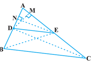
We need to prove that ![]()
Let us join BE and CD and then draw DM ⊥ AC and EN ⊥ AB.
![]()
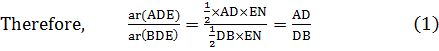
Recall from Class IX, that area of ΔADE is denoted as are
![]()
![]()
![]()
Note that ∆BDE and DEC are on the same base DE and between the same parallels BC and DE.
So, ar(BDE) = ar(DEC)
Therefore, from (1), (2) and (3), we have:
![]()
Criteria for Similarity of Triangles
- Books Name
- Kaysons Academy Maths Foundation Book
- Publication
- Kaysons Publication
- Course
- JEE
- Subject
- Maths
Criteria for Similarity of Triangles
In the previous section, we stated that two triangles are similar, if (i) their corresponding angles are equal and (ii) their corresponding sides are in the same ratio (or proportion).
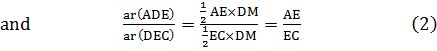
That is, in ΔABC and ΔDEF, if
(i) ∠A = ∠D, ∠B = ∠E, ∠C = ∠F and
![]() Then the two triangles are similar (see Fig).
Then the two triangles are similar (see Fig).
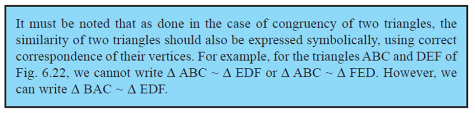
Here, you can see that A corresponds to D, B corresponds to E and C corresponds to F. Symbolically, we write the similarity of these two triangles as ‘ΔABC ~ ΔDEF’ and read it as ‘triangle ABC is similar to triangle DEF’. The symbol ‘~’ stands for ‘is similar to’. Recall that you have used the symbol ‘≅’ for ‘is congruent to’ in Class IX.
Now a natural question arises: For checking the similarity of two triangles, say ABC and DEF, should we always look for all the equality relations of their corresponding angles (∠A = ∠D, ∠B = ∠E, ∠C = ∠F) and all the equality relations of the ratios of their corresponding sides ![]() ? Let us examine. You may recall that in Class IX, you have obtained some criteria for congruency of two triangles involving only three pairs of corresponding parts (or elements) of the two triangles. Here also, let us make an attempt to arrive at certain criteria for similarity of two triangles involving relationship between less numbers of pairs of corresponding parts of the two triangles, instead of all the six pairs of corresponding parts. For this, let us perform the following activity:
? Let us examine. You may recall that in Class IX, you have obtained some criteria for congruency of two triangles involving only three pairs of corresponding parts (or elements) of the two triangles. Here also, let us make an attempt to arrive at certain criteria for similarity of two triangles involving relationship between less numbers of pairs of corresponding parts of the two triangles, instead of all the six pairs of corresponding parts. For this, let us perform the following activity:
Theorem: If in two triangles, sides of one triangle are proportional to (i.e., in the same ratio of) the sides of the other triangle, then their corresponding angles are equal and hence the two triangles are similar. This criterion is referred to as the SSS (Side–Side–Side) similarity criterion for two triangles.
This theorem can be proved by taking two triangles ABC and DEF such that ![]()
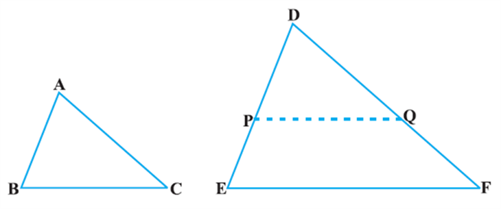
Cut DP = AB and DQ = AC and join PQ.
![]()
![]()
![]()
![]()
![]()
![]()
![]()
Theorem: If one angle of a triangle is equal to one angle of the other triangle and the sides including these angles are proportional, then the two triangles are similar. This criterion is referred to as the SAS (Side–Angle–Side) similarity criterion for two triangles.
As before, this theorem can be proved by taking two triangles ABC and DEF such that ![]() (see Fig). Cut DP = AB, DQ = AC and join PQ.
(see Fig). Cut DP = AB, DQ = AC and join PQ.
Now, PQ || EF and ΔABC ≅ ΔDPQ (How?)
So, ∠A = ∠D, ∠B = ∠P and ∠C = ∠Q
Therefore, ΔABC ~ ΔDEF (Why?)
We now take some examples to illustrate the use of these criteria.
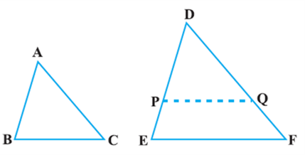
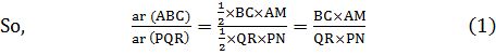
Theorem: The ratio of the areas of two similar triangles is equal to the square of the ratio of their corresponding sides.
Proof : We are given two triangles ABC and PQR such that
ΔABC ~ ΔPQR (see Fig).
We need to prove that ![]()
For finding the areas of the two triangles, we draw altitudes AM to PN of the triangles.
![]()
![]()
![]()
![]()
![]()
![]()
![]()
![]()
![]()
![]()
![]()
Now using (3), we get
![]()
Let us take an example to illustrate the use of this theorem.
Pythagoras Theorem
You are already familiar with the Pythagoras Theorem from your earlier classes. You had verified this theorem through some activities and made use of it in solving certain problems. You have also seen a proof of this theorem in Class IX. Now, we shall prove this theorem using the concept of similarity of triangles. In proving this, we shall make use of a result related to similarity of two triangles formed by the perpendicular to the hypotenuse from the opposite vertex of the right triangle.
Now, let us take a right triangle ABC, right angled at B. Let BD be the perpendicular to the hypotenuse AC (see Fig).
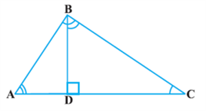
You may note that in ΔADB and ΔABC
∠A = ∠A
and ∠ADB = ∠ABC (Why?)
So, ΔADB ~ ΔABC (How?) (1)
imilarly, ΔBDC ~ ΔABC (How?) (2)
So, from (1) and (2), triangles on both sides of the perpendicular BD are similar to the whole triangle ABC.
Also, since ΔADB ~ ΔABC
and ΔBDC ~ ΔABC
So, ΔADB ~ ΔBDC (From Remark in Section 6.2)
The above discussion leads to the following theorem:
Theorem: If a perpendicular is drawn from the vertex of the right angle of a right triangle to the hypotenuse then triangles on both sides of the perpendicular are similar to the whole triangle and to each other.
Let us now apply this theorem in proving the Pythagoras Theorem:
Theorem: In a right triangle, the square of the hypotenuse is equal to the sum of the squares of the other two sides.
Proof: We are given a right triangle ABC right angled at B. 
We need to prove that AC2 = AB2 + BC2
Let us draw BD ⊥ AC (see Fig.)
Now, ΔADB ~ ΔABC (Theorem)
![]()
![]()
Also, ΔBDC ~ ΔABC (Theorem)
![]()
![]()
Adding (1) and (2),
Theorem: In a triangle, if square of one side is equal to the sum of the squares of the other two sides, then the angle opposite the first side is a right angle.
Proof: Here, we are given a triangle ABC in which AC2 = AB2 + BC2.
We need to prove that ∠B = 90°.
To start with, we construct a ΔPQR right angled at Q such that PQ = AB and QR = BC (see Fig).
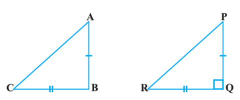
Now, from ΔPQR, we have:
PR2 = PQ2 + QR2 (Pythagoras Theorem, as ∠Q = 90°)
or, PR2 = AB2 + BC2 (By construction) (1)
But AC2 = AB2 + BC2 (Given) (2)
So, AC = PR [From (1) and (2)] (3)
Now, in ΔABC and ΔPQR,
AB = PQ (By construction)
BC = QR (By construction)
AC = PR [Proved in (3) above]
So, ΔABC ≅ ΔPQR (SSS congruence)
Therefore, ∠B = ∠Q (CPCT)
But ∠Q = 90° (By construction)
So, ∠B = 90°
Note: Also see Appendix 1 for another proof of this theorem.
Introduction
- Books Name
- Kaysons Academy Maths Foundation Book
- Publication
- Kaysons Publication
- Course
- JEE
- Subject
- Maths
Chapter:- 8
Introduction to trigonometry
Introduction
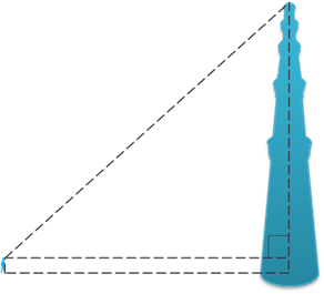
Suppose the students of a school are visiting Qutub Minar. Now, if a student is looking at the top of the Minar, a right triangle can be imagined to be made, as shown in Fig. Can the student find out the height of the Minar, without actually measuring it?
Suppose a girl is sitting on the balcony of her house located on the bank of a river. She is looking down at a flower pot placed on a stair of a temple situated nearby on the other bank of the river. A right triangle is imagined to be made in this situation as shown in Fig. If you know the height at which the person is sitting, can you find the width of the river?

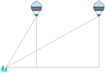
Suppose a hot air balloon is flying in the air. A girl happens to spot the balloon in the sky and runs to her mother to tell her about it. Her mother rushes out of the house to look at the balloon.Now when the girl had spotted the balloon intially it was at point A. When both the mother and daughter came out to see it, it had already travelled to another point B. Can you find the altitude of B from the ground?
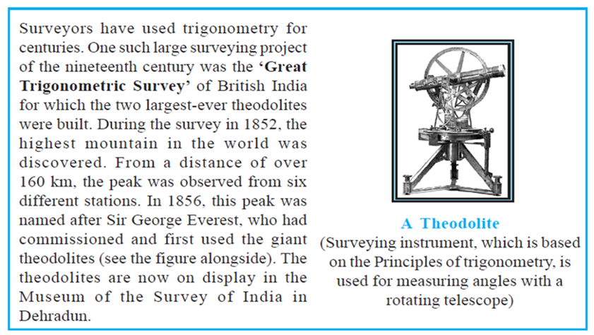
In all the situations given above, the distances or heights can be found by using some mathematical techniques, which come under a branch of mathematics called ‘trigonometry’. The word ‘trigonometry’ is derived from the Greek words ‘tri’ (meaning three), ‘gon’ (meaning sides) and ‘metron’ (meaning measure). In fact, trigonometry is the study of relationships between the sides and angles of a triangle. The earliest known work on trigonometry was recorded in Egypt and Babylon. Early astronomers used it to find out the distances of the stars and planets from the Earth. Even today, most of the technologically advanced methods used in Engineering and Physical Sciences are based on trigonometrical concepts.
In this chapter, we will study some ratios of the sides of a right triangle with respect to its acute angles, called trigonometric ratios of the angle. We will restrict our discussion to acute angles only. However, these ratios can be extended to other angles also. We will also define the trigonometric ratios for angles of measure 0° and 90°. We will calculate trigonometric ratios for some specific angles and establish some identities involving these ratios, called trigonometric identities.
Trigonometric Ratios
In Section 8.1, you have seen some right triangles imagined to be formed in different situations.
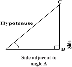
Let us take a right triangle ABC as shown in Fig.
Here, ∠CAB (or, in brief, angle A) is an acute angle. Note the position of the side BC with respect to angle A. it faces ∠A. we call it the side opposite to angle A. AC is the hypotenuse of the right triangle and the side AB is a part of ∠A. so, we call it the side adjacent to angle A.
Note that the position of sides change when you consider angle C in place of A.
You have studied the concept of ‘ratio’ in your earlier classes. We now define certain ratios involving the sides of a right triangle, and call them trigonometric ratios.
The trigonometric ratios of the angle A in right triangle ABC are defined as follows:

Sine of ![]()
![]()
![]()
![]()
![]()
![]()
The ratios defined above are abbreviated as sin A, cos A, tan A, cosec A, sec A and cot A respectively. Note that the ratios cosec A, sec A and cot A are respectively, the reciprocals of the ratios sin A, cos A and tan A.
Also, observe that tan A = 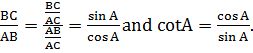
From our observations, it is now clear that the values of the trigonometric ratios of an angle do not vary with the lengths of the sides of the triangle, if the angle remains the same.
Trigonometric Ratios of Some Specific Angles
- Books Name
- Kaysons Academy Maths Foundation Book
- Publication
- Kaysons Publication
- Course
- JEE
- Subject
- Maths
Trigonometric Ratios of Some Specific Angles
From geometry, you are already familiar with the construction of angles of 30°, 45°, 60° and 90°. In this section, we will find the values of the trigonometric ratios for these angles and, of course, for 0°.
Trigonometric Ratios of 45°
In ∆ABC, right-angled at B, if one angle is 45°, then the other angle is also 45°, i.e., ∠A = ∠C = 45°
So, BC = AB (Why?)
Now, Suppose BC = AB = a.
Then by Pythagoras Theorem, AC2 = AB2 + BC2 = a2 + a2 = 2a2,And, therefore, AC = a ![]() .
.
Using the definitions of the trigonometric ratios, we have:
![]()

![]()
![]()
![]()
Trigonometric Ratios of 30° and 60°
Let us now calculate the trigonometric ratios of 30° and 60°. Consider an equilateral triangle ABC. Since each angle in an equilateral triangle is 60°, therefore,
∠A = ∠B = ∠C = 60o
Draw the perpendicular AD from A to the side BC 
Now ∆ABD ≅ ∆ACD (Why?)
Therefore, BD = DC
And ∠BAD = ∠CAD (CPCT)
Now observe that:
∆ABD is a right triangle, right-angled at D with ∠BAD = 30o and ∠ABD = 60o
As you know, for finding the trigonometric ratios, we need to know the lengths of the sides of the triangle. So, let us suppose that AB = 2a.
Then, ![]()
Now, we have:
![]()
![]()
![]()
![]()
Similarly,
![]()
![]()
Trigonometric Ratios of 0° and 90°
Let us see what happens to the trigonometric ratios of angle A, if it is made smaller and smaller in the right triangle ABC (see Fig.), till it becomes zero. As ∠A gets smaller and smaller, the length of the side BC decreases. The point C gets closer to point B, and finally when ∠A becomes very close to 0°, AC becomes almost the same as AB.
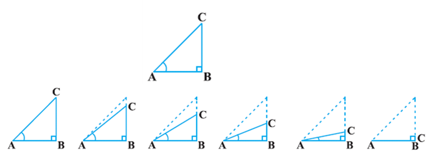
When ∠A is very close to 0o, BC gets very close to 0 and so the value of ![]() is very close to 0. Also, when ∠A is very close to 00, AC is nearly the same as AB and so the value of
is very close to 0. Also, when ∠A is very close to 00, AC is nearly the same as AB and so the value of ![]()
This helps us to how we can define the values of sin A cos A when A = 00. We define: sin 00 = 0 and cos 00 = 1.
Using these, we have
![]()
![]()
Now, let us see what happens to the trigonometric ratios of ∠A, when it is made larger and larger in ∠ABC till it becomes 90°. As ∠A gets larger and larger, ∠C gets smaller and smaller. Therefore, as in the case above, the length of the side AB goes on decreasing. The point A gets closer to point B. Finally when ∠A is very close to 90°, ∠C becomes very close to 0° and the side AC almost coincides with side BC.

When ∠C is very close to 0o, ∠A is very close to 90o, side AC is nearly the same as side BC, and so sin A is very close to 1. Also when ∠A is very close to 90o, ∠C is very close to 0o, and the side AB is nearly zero, so cos A is very close to 0.
So, we define:
sin 90o = 1 and cos 90o = 0.
We shall now give the values of all the trigonometric ratios of 0o, 30o 45o, 60o and 90o in Table 8.1, for ready reference
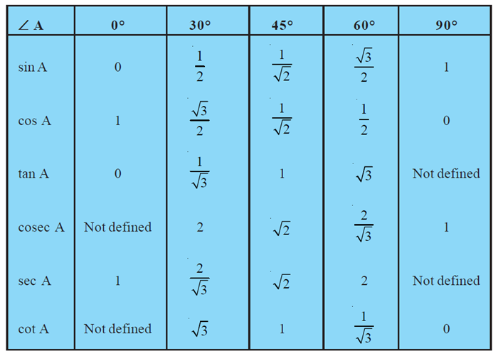
Remark: From the table above you can observe that as ∠A increases from 0o to 90o, sin A increases from 0 to 1 and cos A decreases from 1 to 0.
Trigonometric Ratios of Complementary Angles
- Books Name
- Kaysons Academy Maths Foundation Book
- Publication
- Kaysons Publication
- Course
- JEE
- Subject
- Maths
Trigonometric Ratios of Complementary Angles
Recall that two angles are said to be complementary if their sum equals 90°. In ∠ABC, right-angled at B, do you see any pair of complementary angles?
Since ∠A + ∠C = 90o, they form such a pair. We have:


Now let us write the trigonometric ratios for ∠C = 90o - ∠A.
For convenience, we shall write 90o – A instead of 90o - ∠A.
What would be the side opposite and the side adjacent to the angle 90o – A?
You will find that AB is the side opposite and BC is the side adjacent to the angle
90o – A. Therefore,

Now, compare the ratios in (1) and (2). Observe that:
![]()
![]()
So,
![]()
![]()
![]()
For all values of angle A lying between 0o and 90o. Check whether this holds for A = 0o or A = 90o.
Trigonometric Identities
You may recall that an equation is called an identity when it is true for all values of the variables involved. Similarly, an equation involving trigonometric ratios of an angle is called a trigonometric identity, if it is true for all values of the angle (s) involved.
In this section, we will prove one trigonometric identity, and use it further to prove other useful trigonometric identities.
In ∆ABC, right-angled at B, we have:
AB2 + BC2 = AC2 (1)
Dividing each term of (1) by AC2, we get
![]()
i.e., ![]()
i.e., cos2 A + sin2 A = 1 (2)

This is true for all A such that 0o ≤ A ≤ 90o. So this is a trigonometric identity.
Let us now divide (1) by AB2. We get
![]()
Or, ![]()
i.e., 1 + tan2 A = sec2 A (3)
Is this equation true for A = 0o? Yes, it is. What about A = 90o? Well, tan A and sec A are not defined for A = 90o. So, (3) is true for all A such that 0o ≤ A < 90o.
Let us see what we get on dividing (1) by BC2. We get
![]()
i.e., ![]()
i.e., cot2 A + 1 = cosec2 A (4)
Introduction
- Books Name
- Kaysons Academy Maths Foundation Book
- Publication
- Kaysons Publication
- Course
- JEE
- Subject
- Maths
Chapter -6
STATISTICS
Introduction
In fact, you went a step further by studying certain numerical representatives of the ungrouped data, also called measures of central tendency, namely, mean, median and mode. In this chapter, we shall extend the study of these three measures, i.e., mean, median and mode from ungrouped data to that of grouped data. We shall also discuss the concept of cumulative frequency, the cumulative frequency distribution and how to draw cumulative frequency curves, called ogives.
Mean of Grouped Data
The mean (or average) of observations, as we know, is the sum of the values of all the observations divided by the total number of observations. From Class IX, recall that if x1, x2,…., xn are observations with respective frequencies f1, f2, …., fnxn, then this means observation x1 occurs f1 times, x2 occurs f2 times, and so on.
Now, the sum of the values of all the observations = f1x1 + f2x2 + … + fnxn, and the number of observations = f1 + f2 + … + fn.
So, the mean ![]() of the data is given by
of the data is given by
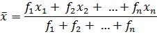
Recall that we can write this in short form by using the Greek letter ∑ (capital sigma) which means summation. That is,
![]()
Which, more briefly, is written as ![]() if it is understood that I varies from 1 to n.
if it is understood that I varies from 1 to n.
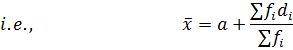
So, from Table 14.4, the mean of the deviations, ![]()
Now, let us find the relation between
Since in obtaining di, we subtracted ‘a’ from each xi, so, in order to get the mean ![]() we need to add ‘a’ to
we need to add ‘a’ to ![]() . This can be explained mathematically as:
. This can be explained mathematically as:
Mean of deviations, ![]()
So, ![]()
![]()
![]()
![]()
Median of Grouped Data
As you have studied in Class IX, the median is a measure of central tendency which gives the value of the middle-most observation in the data. Recall that for finding the median of ungrouped data, we first arrange the data values of the observations in ascending order. Then, if n is odd, the median is the ![]() observation. And, if is even, then the
observation. And, if is even, then the ![]()
After finding the median class, we use the following formula for calculating the median.
![]()
Where l = lower limit of median class,
n = Number of observations,
cf = Cumulative frequency of class preceding the median class,
f = Frequency of median class,
h = Class size (assuming class size to be equal).
Remarks:
1. There is an empirical relationship between the three measures of central tendency:
2 Median = Mode + 2 Mean
3. The median of grouped data with unequal class sizes can also be calculated. However, we shall not discuss it here.
Mode of Grouped Data
- Books Name
- Kaysons Academy Maths Foundation Book
- Publication
- Kaysons Publication
- Course
- JEE
- Subject
- Maths
Mode of Grouped Data
Recall from Class IX, a mode is that value among the observations which occurs most often, that is, the value of the observation having the maximum frequency. Further, we discussed finding the mode of ungrouped data. Here, we shall discuss ways of obtaining a mode of grouped data. It is possible that more than one value may have the same maximum frequency. In such situations, the data is said to be multimodal. Though grouped data can also be multimodal, we shall restrict ourselves to problems having a single mode only.
![]()
Where l = lower limit of the modal class,
h = size of the class interval (assuming all class sizes to be equal),
f1 = frequency of the modal class,
f0 = frequency of the class preceding the modal class,
f2 = frequency of the class succeeding the modal class.
Let us consider the following examples to illustrate the use of this formula.
Graphical Representation of Cumulative Frequency Distribution
As we all know, pictures speak better than words. A graphical representation helps us in understanding given data at a glance. In Class IX, we have represented the data through bar graphs, histograms and frequency polygons. Let us now represent a cumulative frequency distribution graphically.
For example, let us consider the cumulative frequency distribution given in Table 14.13.
Recall that the values 10, 20, 30,. . ., 100 are the upper limits of the respective class intervals. To represent the data in the table graphically, we mark the upper limits of the class intervals on the horizontal axis (x-axis) and their corresponding cumulative frequencies on the vertical axis (y-axis), choosing a convenient scale. The scale may not be the same on both the axis. Let us now plot the points corresponding to the ordered pairs given by (upper limit, corresponding cumulative frequency), i.e., (10, 5), (20, 8), (30, 12), (40, 15), (50, 18), (60, 22), (70, 29), (80, 38), (90, 45), (100, 53) on a graph paper and join them by a free hand smooth curve. The curve we get is called a cumulative frequency curve, or an ogive (of the less than type).

Introduction
- Books Name
- Kaysons Academy Maths Foundation Book
- Publication
- Kaysons Publication
- Course
- JEE
- Subject
- Maths
Chapter-7
Quadratic equations
Introduction
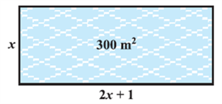
In Chapter 2, you have studied different types of polynomials. One type was the quadratic polynomial of the form ax2 + bx + c, a ≠ 0. When we equate this polynomial to zero, we get a quadratic equation. Quadratic equations come up when we deal with many real-life situations. For instance, suppose a charity trust decides to build a prayer hall having a carpet area of 300 square metres with its length one metre more than twice its breadth. What should be the length and breadth of the hall? Suppose the breadth of the hall is x metres. Then, its length should be (2x + 1) metres. We can depict this information pictorially as shown in Fig.
Now, area of the hall = (2x + 1). xm2 = (2x2 + x) m2
So, 2x2 + x = 300 (Given)
Therefore, 2x2 + x – 300 = 0
So, the breadth of the hall should satisfy the equation 2x2 + x – 300 = 0 which is a quadratic equation.
Quadratic Equations
A quadratic equation in the variable x is an equation of the form ax2 + bx + c = 0, where a, b, c are real numbers, a ≠ 0. For example, 2x2 + x – 300 = 0 is a quadratic equation.
Similarly, 2x2 – 3x + 1 = 0, 4x – 3x2 + 2 = 0 and 1 – x2 + 300 = 0 are also quadratic equations.
In fact, any equation of the form p(x) = 0, where p(x) is a polynomial of degree 2, is a quadratic equation. But when we write the terms of p(x) in descending order of their degrees, then we get the standard form of the equation. That is, ax2 + bx + c = 0, a ≠ 0 is called the standard form of a quadratic equation.
Quadratic equations arise in several situations in the world around us and in different fields of mathematics.
Relationship between Zeroes and Coefficients of a Polynomial
In general, a real number α is called a root of the quadratic equation ax2 + bx + c = 0, a ≠ 0 if a α2 + bα + c = 0. We also say that x = α is a solution of the quadratic equation, or that α satisfies the quadratic equation. Note that the zeroes of the quadratic polynomial ax2 + bx + c and the roots of the quadratic equation ax2 + bx + c = 0 are the same.
Note:- That we have found the roots of 2x2 – 5x + 3 = 0 by factorizing 2x2 – 5x + 3 into two linear factors and equating each factor to zero.
Solution of a Quadratic Equation by Completing the Square
- Books Name
- Kaysons Academy Maths Foundation Book
- Publication
- Kaysons Publication
- Course
- JEE
- Subject
- Maths
Solution of a Quadratic Equation by Completing the Square
In the previous section, you have learnt one method of obtaining the roots of a quadratic equation. In this section, we shall study another method.
Consider the following situation:
The product of Sunita’s age (in years) two years ago and her age four years from now is one more than twice her present age. What is her present age?
To answer this, let her present age (in years) be x. Then the product of her ages two years ago and four years from now is (x – 2) (x + 4).
Now consider the quadratic equation (x + 2)2 – 9 = 0. To solve it, we can write it as (x + 2)2 = 9. Taking square roots, we get x + 2 = 3 or x + 2 = – 3.
Therefore, x = 1 or x = –5
So, the roots of the equation (x + 2)2 – 9 = 0 are 1 and – 5.
In both the examples above, the term containing x is completely inside a square, and we found the roots easily by taking the square roots. But, what happens if we are asked to solve the equation x2 + 4x – 5 = 0? We would probably apply factorisation to do so, unless we realise (somehow!) that x2 + 4x – 5 = (x + 2)2 – 9.
So, solving x2 + 4x – 5 = 0 is equivalent to solving (x + 2)2 – 9 = 0, which we have seen is very quick to do. In fact, we can convert any quadratic equation to the form (x + a)2 – b2 = 0 and then we can easily find its roots. Let us see if this is possible.
Look at Fig.
In this figure, we can see how x2 + 4x is being converted to (x + 2)2 – 4.
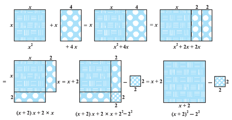
So, x2 + 4x – 5 = 0 can be written as (x + 2)2 – 9 = 0 by this process of completing the square. This is known as the method of completing the square.
In brief, this can be shown as follows:
![]()
![]()
![]()
![]()
Consider now the equation 3x2 – 5x + 2 = 0. Note that the coefficient of x2 is not a perfect square. So, we multiply the equation throughout by 3 to get
![]()
![]()
![]()
![]()
So, 9x2 – 15x + 6 = 0 can be written as
![]()
![]()
So, the solution of 9x2 – 15x + 6 = 0 are the same as those of ![]()
![]()
(We can also write this as ![]() where ‘
where ‘
![]()
![]()
![]()
Consider the quadratic equation ![]() Dividing throughout by a,
Dividing throughout by a,
We get ![]()
![]()
![]()
So, the roots of the given equation are the same as those of
![]()
![]()
![]()
So, the roots of ax2 + bx + c = 0 are ![]()
Equation will have no real roots. (Why?)
Thus, if ![]() then the roots of the quadratic equation ax2 + bx + = 0 are given by
then the roots of the quadratic equation ax2 + bx + = 0 are given by ![]()
This formula for finding the roots of a quadratic equation is known as the quadratic formula.
Nature of Roots
In the previous section, you have seen that the roots of the equation ax2 + bx + c = 0 are given by
![]()
If b2 – 4ac > 0, we get two distinct real roots ![]()
![]()
So, the roots of the equation ax2 + bx + c = 0 are both ![]()
Therefore, we say that the quadratic equation ax2 + bx + c = 0 has two equal real roots in this case.
If b2 – 4ac < 0, then there is no real number whose square is b2 – 4ac. Therefore, there are no real roots for the given quadratic equation in this case.
Since b2 – 4ac determines whether the quadratic equation ax2 + bx + c = 0 has real roots or not, b2 – 4ac is called the discriminant of this quadratic equation.
So, a quadratic equation ax2 + bx + c = 0 has
(i) Two distinct real roots, if b2 – 4ac > 0,
(ii) Two equal real roots, if b2 – 4ac = 0,
(iii) No real roots, if b2 – 4ac < 0.
Introduction
- Books Name
- Kaysons Academy Maths Foundation Book
- Publication
- Kaysons Publication
- Course
- JEE
- Subject
- Maths
CHAPTER -8
ARITHMETIC PROGRESSIONS
Introduction
You must have observed that in nature, many things follow a certain pattern, such as the petals of a sunflower, the holes of a honeycomb, the grains on a maize cob, the spirals on a pineapple and on a pine cone etc.
We now look for some patterns which occur in our day-to-day life. Some such examples are:
(i) Reena applied for a job and got selected. She has been offered a job with a starting monthly salary of 8000, with an annual increment of 500 in her salary. Her salary (in ) for the 1st, 2nd, 3rd, . . . years will be, respectively
8000, 8500, 9000, . . . .
(ii) The lengths of the rungs of a ladder decrease uniformly by 2 cm from bottom to top (see Fig. 5.1). The bottom rung is 45 cm in length. The lengths (in cm) of the 1st, 2nd, 3rd, . . ., 8th rung from the bottom to the top are, respectively
45, 43, 41, 39, 37, 35, 33, 31
(iii) In a savings scheme, the amount becomes ![]() times of itself after every 3 years.
times of itself after every 3 years.
The maturity amount (in) of an investment 8000 after 3, 6, 9 and 12 years will be, respectively:
10000, 12500, 15625, 19531.25

Arithmetic Progressions
Consider the following lists of numbers:
(i) 1, 2, 3, 4, . . .
(ii) 100, 70, 40, 10, . . .
(iii) – 3, –2, –1, 0, . . .
(iv) 3, 3, 3, 3, . . .
(v) –1.0, –1.5, –2.0, –2.5, . . .
Each of the numbers in the list is called a term.
Given a term, can you write the next term in each of the lists above? If so, how will you write it? Perhaps by following a pattern or rule. Let us observe and write the rule.
In (i), each term is 1 more than the term preceding it. In (ii), each term is 30 less than the term preceding it.
In (iii), each term is obtained by adding 1 to the term preceding it.
In (iv), all the terms in the list are 3, i.e., each term is obtained by adding (or subtracting) 0 to the term preceding it.
In (v), each term is obtained by adding – 0.5 to (i.e., subtracting 0.5 from) the term preceding it.
In all the lists above, we see that successive terms are obtained by adding a fixed number to the preceding terms. Such list of numbers is said to form an Arithmetic Progression (AP).
So, an arithmetic progression is a list of numbers in which each term is obtained by adding a fixed number to the preceding term except the first term.
This fixed number is called the common difference of the AP. Remember that it can be positive, negative or zero.
Let us denote the first term of an AP by a1, second term by a2, …..,nth term by an and the common difference by d. then the AP becomes a1, a2, a3, ….., an.
So, a2 – a1 = a3 – a2 = … = an – an – 1= d.
Some more examples of AP are:
(a) The heights (in cm) of some students of a school standing in a queue in the morning assembly are 147, 148, 149, . . ., 157.
(b) The minimum temperatures (in degree celsius) recorded for a week in the month of January in a city, arranged in ascending order are
– 3.1, – 3.0, – 2.9, – 2.8, – 2.7, – 2.6, – 2.5
(c) The balance money (in) after paying 5 % of the total loan of 1000 every month is 950, 900, 850, 800, . . ., 50.
(d) The cash prizes (in) given by a school to the toppers of Classes I to XII are, respectively, 200, 250, 300, 350, . . ., 750.
(e) The total savings (in) after every month for 10 months when 50 are saved each month are 50, 100, 150, 200, 250, 300, 350, 400, 450, 500.
It is left as an exercise for you to explain why each of the lists above is an AP.
You can see that
a, a + d, a + 2d, a + 3d, . . .
Represents an arithmetic progression where a is the first term and d the common difference. This is called the general form of an AP.
Note that in examples (a) to (e) above, there are only a finite number of terms. Such an AP is called a finite AP. Also note that each of these Arithmetic Progressions (APs) has a last term. The APs in examples (i) to (v) in this section are not finite APs and so they are called infinite Arithmetic Progressions. Such APs do not have a last term.
nth Term of an AP
Let us consider the situation again, given in Section 5.1 in which Reena applied for a job and got selected. She has been offered the job with a starting monthly salary of 8000, with an annual increment of 500. What would be her monthly salary for the fifth year?
Let a1, a2, a3,…be an AP whose first term a1 is a and the common difference is d.
Then,
The second term a2 = a + d = a + (2 – 1) d
The third term a3 = a2 + d = (a + d) = a + 2d = a + (3 – 1) d
The fourth term a4 = a3 + d = (a + 2d) + d = a + 3d = a + (4 – 1) d…………..
Looking at the pattern, we can say that the nth term an = a + (n – 1) d.
So, the nth term an of the AP with first term a and common difference d is given by
an = a + (n – 1) d.
an is also called the general term of the AP. If there are m terms in the AP, then am represents the last term which is sometimes also denoted by l.
Sum of First n Terms of an AP
- Books Name
- Kaysons Academy Maths Foundation Book
- Publication
- Kaysons Publication
- Course
- JEE
- Subject
- Maths
Sum of First n Terms of an AP
Let us consider the situation again given in Section 5.1 in which Shakila put ![]() 100 into her daughter’s money box when she was one year old,
100 into her daughter’s money box when she was one year old, ![]() 150 on her second birthday,
150 on her second birthday, ![]() 200 on her third birthday and will continue in the same way. How much money will be collected in the money box by the time her daughter is 21 years old?
200 on her third birthday and will continue in the same way. How much money will be collected in the money box by the time her daughter is 21 years old?

Here, the amount of money (in ![]() ) put in the money box on her first, second, third, fourth . . . birthday were respectively 100, 150, 200, 250, . . . till her 21st birthday. To find the total amount in the money box on her 21st birthday, we will have to write each of the 21 numbers in the list above and then add them up. Don’t you think it would be a tedious and time consuming process? Can we make the process shorter? This would be possible if we can find a method for getting this sum. Let us see.
) put in the money box on her first, second, third, fourth . . . birthday were respectively 100, 150, 200, 250, . . . till her 21st birthday. To find the total amount in the money box on her 21st birthday, we will have to write each of the 21 numbers in the list above and then add them up. Don’t you think it would be a tedious and time consuming process? Can we make the process shorter? This would be possible if we can find a method for getting this sum. Let us see.
We consider the problem given to Gauss (about whom you read in Chapter 1), to solve when he was just 10 years old. He was asked to find the sum of the positive integers from 1 to 100. He immediately replied that the sum is 5050. Can you guess how did he do? He wrote:
S = 1 + 2 + 3 + . . . + 99 + 100
And then, reversed the numbers to write
S = 100 + 99 + . . . + 3 + 2 + 1
Adding these two, he got
2S = (100 + 1) + (99 + 2) + . . . + (3 + 98) + (2 + 99) + (1 + 100)
= 101 + 101 + . . . + 101 + 101 (100 times)
So, ![]() i.e., the sum = 5050.
i.e., the sum = 5050.
We will now use the same technique to find the sum of the first n terms of an AP:
a, a + d, a + 2d, . . .
The nth term of this AP is a + (n – 1) d. Let S denote the sum of the first n terms of the AP. We have
S = a + (a + d) + (a + 2d) + . . . + [a + (n – 1) d] (1)
Rewriting the terms in reverse order, we have
= [a + (n – 1) d] + [a + (n – 2) d] + . . . + (a + d) + a (2)
On adding (1) and (2), term-wise. We get
![]()
or, 2S = n [2a + (n – 1) d] (Since, there are n terms)
or, ![]()
So, the sum of the first n terms of an AP is given by
![]()
We can also write this as ![]()
i.e., ![]() (3)
(3)
Now, if there are only n terms in an AP, then an = l, the last term. From (3), we see that
![]() (4)
(4)
Introduction
- Books Name
- Kaysons Academy Maths Foundation Book
- Publication
- Kaysons Publication
- Course
- JEE
- Subject
- Maths
Chapter:- 9
COORDINATE GEOMETRY
Introduction
In Class IX, you have studied that to locate the position of a point on a plane, we require a pair of coordinate axes. The distance of a point from the y-axis is called its x-coordinate, or abscissa. The distance of a point from the x-axis is called its y-coordinate, or ordinate. The coordinates of a point on the x-axis are of the form (x, 0), and of a point on the y-axis are of the form (0, y).
Here is a play for you. Draw a set of a pair of perpendicular axes on a graph paper. Now plot the following points and join them as directed: Join the point A(4, 8) to B(3, 9) to C(3, 8) to D(1, 6) to E(1, 5) to F(3, 3) to G(6, 3) to H(8, 5) to I(8, 6) to J(6, 8) to K(6, 9) to L(5, 8) to A. Then join the points P(3.5, 7), Q (3, 6) and R(4, 6) to form a triangle. Also join the points X(5.5, 7), Y(5, 6) and Z(6, 6) to form a triangle. Now join S(4, 5), T(4.5, 4) and U(5, 5) to form a triangle. Lastly join S to the points (0, 5) and (0, 6) and join U to the points (9, 5) and (9, 6). What picture have you got?
Also, you have seen that a linear equation in two variables of the form ax + by + c = 0, (a, b are not simultaneously zero), when represented graphically, gives a straight line. Further, in Chapter 2, you have seen the graph of y = ax2 + bx + c (a ≠ 0), is a parabola. In fact, coordinate geometry has been developed as an algebraic tool for studying geometry of figures. It helps us to study geometry using algebra, and understand algebra with the help of geometry. Because of this, coordinate geometry is widely applied in various fields such as physics, engineering, navigation, seismology and art!
In this chapter, you will learn how to find the distance between the two points whose coordinates are given, and to find the area of the triangle formed by three given points. You will also study how to find the coordinates of the point which divides a line segment joining two given points in a given ratio.
Distance Formula
Let us consider the following situation:
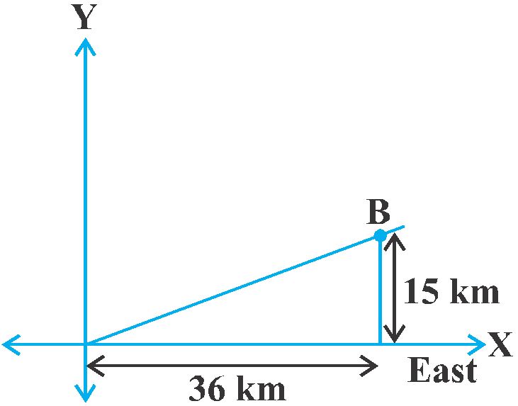
A town B is located 36 km east and 15 km north of the town A. How would you find the distance from town A to town B without actually measuring it. Let us see. This situation can be represented graphically as shown in Fig. You may use the Pythagoras Theorem to calculate this distance.
Now, suppose two points lie on the x-axis.
Can we find the distance between them? For instance, consider two points A(4, 0) and B(6, 0) in Fig. The points A and B lie on the x-axis. From the figure you can see that OA = 4 units and OB = 6 units. Therefore, the distance of B from A, i.e., AB = OB – OA = 6 – 4 = 2 units.

So, if two points lie on the x-axis, we can easily find the distance between them. Now, suppose we take two points lying on the y-axis. Can you find the distance between them. If the points C (0, 3) and D (0, 8) lie on the y-axis, similarly we find that
CD = 8 – 3 = 5 units Next, can you find the distance of A from C (in Fig. 7.2)? Since OA = 4 units and OC = 3 units, the distance of A from C, i.e.,![]() units. Similarly, you can find the distance of B from D = BD = 10 units.
units. Similarly, you can find the distance of B from D = BD = 10 units.
Let us now find the distance between any two points P(x1, y1) and Q (x2, y2). Draw R and QS perpendicular to the x-axis. A perpendicular from the point P on QS is rawn to meet it at the point T.
Then, OR = x1, OS = x2. So, RS = x2 – x1 = PT.
Also, SQ = y2, ST = PR = y1. So, QT = y2 – y1.
Now, applying the Pythagoras theorem in ∆PTQ, we get
PQ2 = PT2 + QT2
= (x2 – x1)2 + (y2 – y1)2
Therefore,
![]()
Note that since distance is always non-negative, we take only the positive square root. So, the distance between the points P(x1, y1) and Q(x2, y2) is
![]()
Which is called the distance formula.
Remarks:
1. In particular, the distance of a point P(x, y) from the origin O (0, 0) is given by
![]()
2. We can also write, ![]()
Section Formula
Let us recall the situation in Section 7.2. Suppose a telephone company wants to position a relay tower at P between A and B is such a way that the distance of the tower from B is twice its distance from A. If P lies on AB, it will divide AB in the ratio 1 : 2. If we take A as the origin O, and 1 km as one unit on both the axis, the coordinates of B will be (36, 15). In order to know the position of the tower, we must know the coordinates of P. How do we find these coordinates?

Let the coordinates of P be (x, y). Draw perpendiculars from P and B to the x-axis, meeting it in D and E, respectively. Draw PC perpendicular to BE. Then, by the AA similarity criterion, studied in Chapter 6, ∆POD and ∆BPC are similar.
Therefore, ![]()
So, ![]()
These equations give x = 12 and y = 5.
You can check that P(12, 5) meets the condition that OP : PB = 1 : 2.
Now let us use the understanding that you may have developed through this example to obtain the general formula.
Consider any two points A(x1, y1) and B(x2, y2) and assume that P(x, y) divides AB internally in the ratio m1 : m2, i.e.,![]()
Draw AR, PS and BT perpendicular to the x-axis. Draw AQ and PC parallel to the x-axis. Then, by the AA similarity criterion,
∆PAQ ~ ∆BPC
Therefore, ![]() (1)
(1)
Now, AQ = RS = OS – OR = x – x1
PC = ST = OT – OS = x2 – x
PQ = PS – QS = PS – AR = y – y1
BC = BT – CT = BT – PS = y2 – y
Substituting these values in (1), we get
![]()
Taking ![]()
Similarly, taking
![]()
So, the coordinates of the point P(x, y) which divides the line segment joining the points A(x1, y1) and B(x2, y2), internally, in the ratio m1 : m2 are
![]() (2)
(2)
This is known as the section formula.
This can also be derived by drawing perpendiculars from A, P and B on the y-axis and proceeding as above.
If the ratio in which P divides AB is k : 1, then the coordinates of the point P will be
![]()
Special Case: The mid-point of a line segment divides the line segment in the ratio 1 : 1. Therefore, the coordinates of the mid-point P of the join of the points A(x1, y1) and B(x2, y2) is
![]()
Let us solve a few examples based on the section formula.
Area of a Triangle
In your earlier classes, you have studied how to calculate the area of a triangle when its base and corresponding height (altitude) are given. You have used the formula:
![]()
In Class IX, you have also studied Heron’s formula to find the area of a triangle. Now, if the coordinates of the vertices of a triangle are given, can you find its area? Well, you could find the lengths of the three sides using the distance formula and then use Heron’s formula. But this could be tedious, particularly if the lengths of the sides are irrational numbers. Let us see if there is an easier way out.
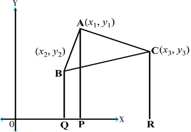
Let ABC be any triangle whose vertices are A(x1, y1), B(x2, y2) and C(x3, y3). Draw AP,
BQ and CR perpendiculars from A, B and C, Respectively, to the x-axis. Clearly ABQP,
APRC and BQRC are all trapzia.
Now, from Fig. it is clear that
Area of ∆ABC = area of trapezium ABQP + area of trapezium APRC – area of trapezium BQRC.
You also know that the Area of a trapezium = ![]() (sum of parallel sides) (distance between them)
(sum of parallel sides) (distance between them)
Therefore,
Area of ∆ABC =![]()
![]()
![]()
Thus, the area of ∆ABC is the numerical value of the expression
![]()
Let us consider a few examples in which we make use of this formula.
Introduction
- Books Name
- Kaysons Academy Maths Foundation Book
- Publication
- Kaysons Publication
- Course
- JEE
- Subject
- Maths
Chapter -10
Some applications of trigonometry
Introduction
In the previous chapter, you have studied about trigonometric ratios. In this chapter, you will be studying about some ways in which trigonometry is used in the life around you Trigonometry is one of the most ancient subjects studied by scholars all over the world As we have said in Chapter 8, trigonometry was invented because its need arose in astronomy. Since then the astronomers have used it, for instance, to calculate distances from the Earth to the planets and stars. Trigonometry is also used in geography and in navigation. The knowledge of trigonometry is used to construct maps, determine the position of an island in relation to the longitudes and latitudes.
In this chapter, we will see how trigonometry is used for finding the heights and distances of various objects, without actually measuring them.
Heights and Distances
Let us consider Fig of previous chapter, which is redrawn below in Fig.
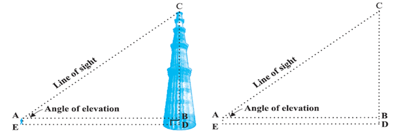
In this figure, the line AC drawn from the eye of the student to the top of the minar is called the line of sight. The student is looking at the top of the minar. The angle BAC, so formed by the line of sight with the horizontal, is called the angle of elevation of the top of the minar from the eye of the student.
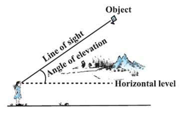
Thus, the line of sight is the line drawn from the eye of an observer to the point in the object viewed by the observer. The angle of elevation of the point viewed is the angle formed by the line of sight with the horizontal when the point being viewed is above the horizontal level, i.e., the case when we raise our head to look at the object (see Fig).
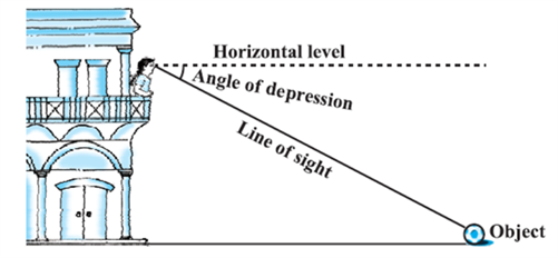
Now, consider the situation given in Fig. The girl sitting on the balcony is looking down at a flower pot placed on a stair of the temple. In this case, the line of sight is below the horizontal level. The angle so formed by the line of sight with the horizontal is called the angle of depression.
Thus, the angle of depression of a point on the object being viewed is the angle formed by the line of sight with the horizontal when the point is below the horizontal level, i.e., the case when we lower our head to look at the point being viewed (see Fig).
Now, you may identify the lines of sight, and the angles so formed in Fig. Are they angles of elevation or angles of depression?
Let us refer to Fig. again. If you want to find the height CD of the minar without actually measuring it, what information do you need? You would need to know the following:
(i) The distance DE at which the student is standing from the foot of the minar
(ii) The angle of elevation, ∠BAC, of the top of the minar
(iii) The height AE of the student.
Assuming that the above three conditions are known, how can we determine the height of the minar?
In the figure, CD = CB + BD. Here, BD = AE, which is the height of the student.
To find BC, we will use trigonometric ratios of ∠BAC or ∠A.
In D ABC, the side BC is the opposite side in relation to the known ∠A. Now, which of the trigonometric ratios can we use? Which one of them has the two values that we have and the one we need to determine? Our search narrows down to using either tan A or cot A, as these ratios involve AB and BC.
![]() which on solving would give as BC.
which on solving would give as BC.
By adding AE to BC, you will the height of the minar.
Now let us explain the process, we have just discussed, by solving some problems.
Introduction
- Books Name
- Kaysons Academy Maths Foundation Book
- Publication
- Kaysons Publication
- Course
- JEE
- Subject
- Maths
CHAPTER -11
CIRCLES
Introduction
You have studied in Class IX that a circle is a collection of all points in a plane which are at a constant distance (radius) from a fixed point (centre). You have also studied various terms related to a circle like chord, segment, sector, arc etc. Let us now examine the different situations that can arise when a circle and a line are given in a plane.
So, let us consider a circle and a line PQ. There can be three possibilities given in Fig. below:
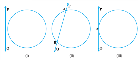
In Fig. (i), the line PQ and the circle have no common point. In this case, PQ is called a non-intersecting line with respect to the circle. In Fig.(ii), there are two common points A and B that the line PQ and the circle have. In this case, we call the line PQ a secant of the circle. In Fig.(iii), there is only one point A which is common to the line PQ and the circle. In this case, the line is called a tangent to the circle.
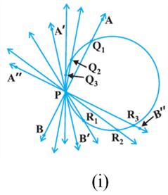
In various positions, the wire intersects the circular wire at P and at another point Q1 or Q2 or Q3, etc. In one position, you will see that it will intersect the circle at the point P only (see position A′B′ of AB). This shows that a tangent exists at the point P of the circle. On rotating further, you can observe that in all other positions of AB, it will intersect the circle at P and at another point, say R1 or R2 or R3, etc. So, you can observe that there is only one tangent at a point of the circle. While doing activity above, you must have observed that as the position AB moves towards the position A′ B′, the common point, say Q1, of the line AB and the circle gradually comes nearer and nearer to the common point P. Ultimately, it coincides with the point P in the position A′B′ of A′′B′′. Again note, what happens if ‘AB’ is rotated rightwards about P? The common point R3 gradually comes nearer and nearer to P and ultimately coincides with P. So, what we see is:
The tangent to a circle is a special case of the secant, when the two end points of its corresponding chord coincide.
Activity 2: On a paper, draw a circle and a secant PQ of the circle. Draw various lines parallel to the secant on both sides of it. You will find that after some steps, the length of the chord cut by the lines will gradually decrease, i.e., the two points of intersection of the line and the circle are coming closer and closer [see Fig (ii)]. In one case, it becomes zero on one side of the secant and in another case, it becomes zero on the other side of the secant. See the positions P′Q′ and P′′Q′′ of the secant in Fig (ii). These are the tangents to the circle parallel to the given secant PQ. This also helps you to see that there cannot be more than two tangents parallel to a given secant.
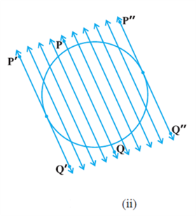
This activity also establishes, what you must have observed, while doing Activity 1, namely, a tangent is the secant when both of the end points of the corresponding chord coincide.
The common point of the tangent and the circle is called the point of contact [the point A in Fig (iii)] and the tangent is said to touch the circle at the common point.
Number of Tangents from a Point on a Circle
To get an idea of the number of tangents from a point on a circle, let us perform the following activity:
Activity 3: Draw a circle on a paper. Take a point P inside it. Can you draw a tangent to the circle through this point? You will find that all the lines through this point intersect the circle in two points. So, it is not possible to draw any tangent to a circle through a point inside it [see Fig (i)].
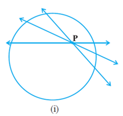
Next take a point P on the circle and draw tangents through this point. You have already observed that there is only one tangent to the circle at such a point [see Fig (ii)].
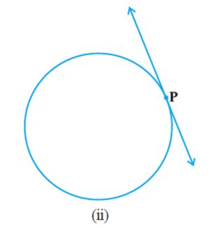
Finally, take a point P outside the circle and try to draw tangents to the circle from this point. What do you observe? You will find that you can draw exactly two tangents to the circle through this point [see Fig (iii)].
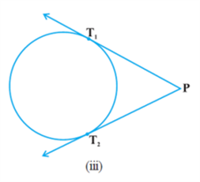
We can summaries these facts as follows:
Case 1: There is no tangent to a circle passing through a point lying inside the circle.
Case 2: There is one and only one tangent to a circle passing through a point lying on the circle.
Case 3: There are exactly two tangents to a circle through a point lying outside the circle. In Fig (iii), T1and T2 are the points of contact of the tangents PT1 and PT2 respectively. he length of the segment of the tangent from the external point P and the point of contact with the circle is called the length of the tangent from the point P to the circle.
Introduction
- Books Name
- Kaysons Academy Maths Foundation Book
- Publication
- Kaysons Publication
- Course
- JEE
- Subject
- Maths
Chapter -12
AREAS RELATED TO CIRCLES
Introduction
You are already familiar with some methods of finding perimeters and areas of simple plane figures such as rectangles, squares, parallelograms, triangles and circles from your earlier classes. Many objects that we come across in our daily life are related to the circular shape in some form or the other. Cycle wheels, wheel barrow (thela), dartboard, round cake, papad, drain cover, various designs, bangles, brooches, circular paths, washers, flower beds, etc. are some examples of such objects (see Fig). So, the problem of finding perimeters and areas related to circular figures is of great practical importance. In this chapter, we shall begin our discussion with a review of the concepts of perimeter (circumference) and area of a circle and apply this knowledge in finding the areas of two special ‘parts’ of a circular region (or briefly of a circle) known as sector and segment. We shall also see how to find the areas of some combinations of plane figures involving circles or their parts Fig.
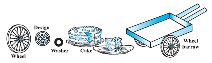
Perimeter and Area of a Circle — A Review
Recall that the distance covered by travelling once around a circle is its perimeter, usually called its circumference. You also know from your earlier classes, that circumference of a circle bears a constant ratio with its diameter. This constant ratio is denoted by the Greek letter π (read as ‘pi’). In other words,
![]()
![]()
![]()
![]()
Areas of Sector and Segment of a Circle
You have already come across the terms sector and segment of a circle in your earlier classes. Recall that the portion (or part) of the circular region enclosed by two radii and the corresponding arc is called a sector of the circle and the portion (or part) of the circular region enclosed between a chord and the corresponding arc is called a segment of the circle. Thus, in Fig. Shaded region OAPB is a sector of the circle with centre O. ∠ AOB is called the angle of the sector. Note that in this figure, unshaded region OAQB is also a sector of the circle. For obvious reasons, OAPB is called the minor sector and OAQB is called the major sector. You can also see that angle of the major sector is 360° – ∠ AOB.
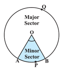
Now, look at Fig, in which AB is a chord of the circle with centre O. So, shaded region APB is a segment of the circle. You can also note that unshaded region AQB is another segment of the circle formed by the chord AB. For obvious reasons, APB is called the minor segment and AQB is called the major segment.
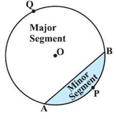
Remark: When we write ‘segment’ and ‘sector’ we will mean the ‘minor segment’ and the ‘minor sector’ respectively, unless stated otherwise. Now with this knowledge, let us try to find some relations (or formulae) to calculate their areas.
Let OAPB be a sector of a circle with centre O and radius r (see Fig). Let the degree measure of ∠AOB be θ. You know that area of a circle (in fact of a circular region or disc) is πr2.
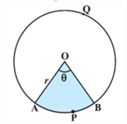
In a way, we can consider this circular region to be a sector forming an angle of 360° (i.e., of degree measure 360) at the centre O. Now by applying the Unitary Method, we can arrive at the area of the sector OAPB as follows:
When degree measure of the angle at the centre is 360, area of the sector = πr2
So, when the degree measure of the angle at the centre is 1, area of the sector ![]()
Therefore, when the degree measure of the angle at the centre is θ, area of the sector ![]()
Thus, we obtain the following relation (or formula) for area of a sector of a circle:
Area of the sector of angle ![]()
Where r is the radius of the circle and θ the angle of the sector in degrees.
Now, a natural question arises: Can we find the length of the arc APB corresponding to this sector? Yes. Again, by applying the Unitary Method and taking the whole length of the circle (of angle 360°) as 2πr, we can obtain the required length of the arc APB as ![]()
So, length of an arc of a sector of angle![]()
Now let us take the case of the area of the segment APB of a circle with centre O and radius r (see Fig). You can see that:
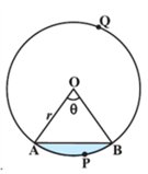
Area of the segment APB = Area of the sector OAPB – Area of D OAB
![]()
Note: From Fig (1) Fig (2), respectively, you can observe that:
Area of the major sector OAQB = πr2 – Area of the minor sector OAPB
And Area of major segment AQB = πr2 – Area of the minor segment APB
Areas of Combinations of Plane Figures
So far, we have calculated the areas of different figures separately. Let us now try to calculate the areas of some combinations of plane figures. We come across these types of figures in our daily life and also in the form of various interesting designs. Flower beds, drain covers, window designs, designs on table covers, are some of such examples.
Introduction
- Books Name
- Kaysons Academy Maths Foundation Book
- Publication
- Kaysons Publication
- Course
- JEE
- Subject
- Maths
Chapter -13
Surface areas and volumes
Introduction
From Class IX, you are familiar with some of the solids like cuboid, cone, cylinder, and sphere (see Fig.). You have also learnt how to find their surface areas and volumes.
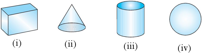
In our day-to-day life, we come across a number of solids made up of combinations of two or more of the basic solids as shown above.
Surface Area of a Combination of Solids
Let us consider the container seen in Fig. How do we find the surface area of such a solid? Now, whenever we come across a new problem, we first try to see, if we can break it down into smaller problems, we have earlier solved. We can see that this solid is made up of a cylinder with two hemispheres stuck at either end. It would look like what we have in Fig., after we put the pieces all together.

If we consider the surface of the newly formed object, we would be able to see only the curved surfaces of the two hemispheres and the curved surface of the cylinder. So, the total surface area of the new solid is the sum of the curved surface areas of each of the individual parts. This gives,
TSA of new solid = CSA of one hemisphere + CSA of cylinder + CSA of other hemisphere
Where TSA, CSA stand for ‘Total Surface Area’ and ‘Curved Surface Area’ respectively.
Let us now consider another situation. Suppose we are making a toy by putting together a hemisphere and a cone. Let us see the steps that we would be going through.
First, we would take a cone and a hemisphere and bring their flat faces together. Here, of course, we would take the base radius of the cone equal to the radius of the hemisphere, for the toy is to have a smooth surface. So, the steps would be as shown in Fig.

At the end of our trial, we have got ourselves a nice round-bottomed toy. Now if we want to find how much paint we would require to colour the surface of this toy, what would we need to know? We would need to know the surface area of the toy, which consists of the CSA of the hemisphere and the CSA of the cone.
So, we can say:
Total surface area of the toy = CSA of hemisphere + CSA of cone
Now, let us consider some examples.
Volume of a Combination of Solids
- Books Name
- Kaysons Academy Maths Foundation Book
- Publication
- Kaysons Publication
- Course
- JEE
- Subject
- Maths
Volume of a Combination of Solids
In the previous section, we have discussed how to find the surface area of solids made up of a combination of two basic solids. Here, we shall see how to calculate their volumes. It may be noted that in calculating the surface area, we have not added the surface areas of the two constituents, because some part of the surface area disappeared in the process of joining them. However, this will not be the case when we calculate the volume. The volume of the solid formed by joining two basic solids will actually be the sum of the volumes of the constituents, as we see in the examples below.
Conversion of Solid from One Shape to Another
We are sure you would have seen candles. Generally, they are in the shape of a cylinder. You may have also seen some candles shaped like an animal (see Fig.). How are the made? If you want a candle of any special shape, you will have to heat the wax in a metal container till it becomes completely liquid. Then you will have to pour it into another container which has the special shape that you want.

For example, take a candle in the shape of a solid cylinder, melt it and pour whole of the molten wax into another container shaped like a rabbit. On cooling, you will obtain a candle in the shape of the rabbit. The volume of the new candle will be the same as the volume of the earlier candle. This is what we have to remember when we come across objects which are converted from one shape to another, or when a liquid which originally filled one container of a particular shape is poured into another container of a different shape or size, as you see in Fig.
To understand what has been discussed, let us consider some examples.
Frustum of a Cone
In section 13.2, we observed objects that are formed when two basic solids were joined together. Let us now do something different. We will take a right circular cone and remove a portion of it. There are so many ways in which we can do this. But one particular case that in which we can do this. But one particular case that we are interested in is the removal of a smaller right circular cone by cutting the given cone by a plane parallel to its base. You must have observed that the glasses (tumblers), in general, used for drinking water, are of this shape. (See Fig.)

Introduction
- Books Name
- Kaysons Academy Maths Foundation Book
- Publication
- Kaysons Publication
- Course
- JEE
- Subject
- Maths
Chapter -14
Probability
Introduction
In Class IX, you have studied about experimental (or empirical) probabilities of events which were based on the results of actual experiments. We discussed an experiment of tossing a coin 1000 times in which the frequencies of the outcomes were as follows:
Head: 455 Tails: 545
Based on this experiment, the empirical probability of a head is ![]() that of getting a tail is 0.545. (Also see Example 1, Chapter 15 of Class IX Mathematics Textbook.) Note that these probabilities are based on the results of an actual experiment of tossing a coin 1000 times. For this reason, they are called experimental or empirical probabilities. In fact, experimental probabilities are based on the results of actual experiments and adequate recordings of the happening of the events. Moreover, these probabilities are only ‘estimates’. If we perform the same experiment for another 1000 times, we may get different data giving different probability estimates.
that of getting a tail is 0.545. (Also see Example 1, Chapter 15 of Class IX Mathematics Textbook.) Note that these probabilities are based on the results of an actual experiment of tossing a coin 1000 times. For this reason, they are called experimental or empirical probabilities. In fact, experimental probabilities are based on the results of actual experiments and adequate recordings of the happening of the events. Moreover, these probabilities are only ‘estimates’. If we perform the same experiment for another 1000 times, we may get different data giving different probability estimates.
In Class IX, you tossed a coin many times and noted the number of times it turned up heads (or tails) (refer to Activities 1 and 2 of Chapter 15). You also noted that as the number of tosses of the coin increased, the experimental probability of getting a head (or tail) came closer and closer to the number ![]() Not only you, but many other Persons from different parts of the world have done this kind of experiment and recorded the number of heads that turned up.
Not only you, but many other Persons from different parts of the world have done this kind of experiment and recorded the number of heads that turned up.
For example, the eighteenth century French naturalist Comte de Buffon tossed a coin 4040 times and got 2048 heads. The experimental probability of getting a head, in this case, was ![]() i.e., 0.507. J.E. Kerrich, from Britain, recorded 5067 heads in 10000 tosses of a coin. The experimental probability of getting a head, in this case, was
i.e., 0.507. J.E. Kerrich, from Britain, recorded 5067 heads in 10000 tosses of a coin. The experimental probability of getting a head, in this case, was ![]() Statistician Karl Pearson spent some more time, making 24000 tosses of a coin. He got 12012 heads, and thus, the experimental probability of a head obtained by him was 0.5005.
Statistician Karl Pearson spent some more time, making 24000 tosses of a coin. He got 12012 heads, and thus, the experimental probability of a head obtained by him was 0.5005.
Now, suppose we ask, ‘What will the experimental probability of a head be if the experiment is carried on upto, say, one million times? Or 10 million times? And so on?’ You would intuitively feel that as the number of tosses increases, the experimental probability of a head (or a tail) seems to be settling down around the number 0.5 , i.e.,
Probability — A Theoretical Approach
Let us consider the following situation:
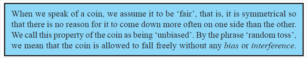
Suppose a coin is tossed at random.
We know, in advance, that the coin can only land in one of two possible ways — either head up or tail up (we dismiss the possibility of its ‘landing’ on its edge, which may be possible, for example, if it falls on sand). We can reasonably assume that each outcome, head or tail, is as likely to occur as the other. We refer to this by saying that the outcomes head and tail, are equally likely.
For another example of equally likely outcomes, suppose we throw a die once. For us, a die will always mean a fair die. What are the possible outcomes? They are 1, 2, 3, 4, 5, 6. Each number has the same possibility of showing up. So the equally likely outcomes of throwing a die are 1, 2, 3, 4, 5 and 6.
Are the outcomes of every experiment equally likely? Let us see.
Suppose that a bag contains 4 red balls and 1 blue ball, and you draw a ball without looking into the bag. What are the outcomes? Are the outcomes — a red ball and a blue ball equally likely? Since there are 4 red balls and only one blue ball, you would agree that you are more likely to get a red ball than a blue ball. So, the outcomes (a red ball or a blue ball) are not equally likely. However, the outcome of drawing a ball of any colour from the bag is equally likely. So, all experiments do not necessarily have equally likely outcomes.
However, in this chapter, from now on, we will assume that all the experiments have equally likely outcomes.
In Class IX, we defined the experimental or empirical probability P(E) of an event E as
![]()
The empirical interpretation of probability can be applied to every event associated with an experiment which can be repeated a large number of times. The requirement of repeating an experiment has some limitations, as it may be very expensive or unfeasible in many situations. Of course, it worked well in coin tossing or die throwing experiments. But how about repeating the experiment of launching a satellite in order to compute the empirical probability of its failure during launching, or the repetition of the phenomenon of an earthquake to compute the empirical probability of a multistoreyed building getting destroyed in an earthquake?
In experiments where we are prepared to make certain assumptions, the repetition of an experiment can be avoided, as the assumptions help in directly calculating the exact (theoretical) probability. The assumption of equally likely outcomes (which is valid in many experiments, as in the two examples above, of a coin and of a die) is one such assumption that leads us to the following definition of probability of an event.
The theoretical probability (also called classical probability) of an event E, written as P(E), is defined as
![]()
Where we assume that the outcomes of the experiment are equally likely.
We will briefly refer to theoretical probability as probability.
This definition of probability was given by Pierre Simon Laplace in 1795.
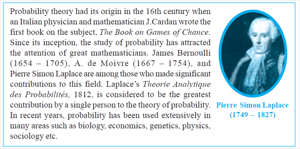
Let us find the probability for some of the events associated with experiments where the equally likely assumption holds.