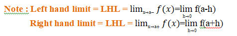
 KRISHNA PUBLICATIONS
1. Concept of Continuity and Algebra of continuous functions
- Books Name
- Mathmatics Book Based on NCERT
- Publication
- KRISHNA PUBLICATIONS
- Course
- CBSE Class 12
- Subject
- Mathmatics
Chapter 5
Continuity and Differentiability
Concept of Continuity and Algebra of continuous functions:
Definition-1:
A function f(x) is said to be continuous at x=a if
![]() =f(a)
=f(a)
A function is said to be continuous on the interval [a,b]
if it is continuous at each point in the interval.
Definition-2:
A function f(x) is said to be continuous at a point x = a, in its domain if the following three conditions are satisfied:
- f(a) exists (i.e. the value of f(a) is finite)
- Limx→a f(x) exists (i.e. the right-hand limit = left-hand limit, and both are finite)
- Limx→a f(x) = f(a)
The function f(x) is said to be continuous in the interval I = [x1,x2] if the three conditions mentioned above are satisfied for every point in the interval I.
If LHL=RHL ,then limit exists.
If LHL=RHL=f(a), then function is continuous at x = a.
Example 1 Given the graph of f(x), shown below, determine if f(x) is continuous at x=−2, x=0, and x=3.
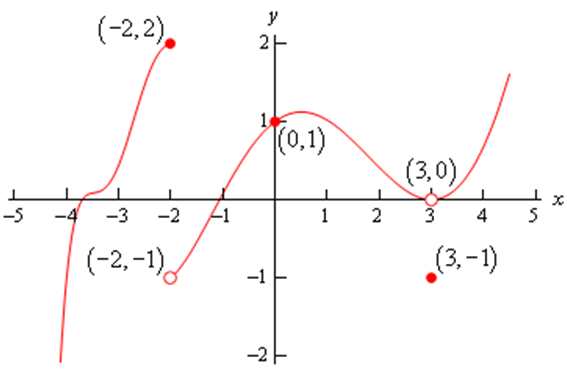
First x=−2.
f(−2)=2 , ![]() doesn't exist.
doesn't exist.
The function value and the limit aren’t the same and so the function is not continuous at this point. This kind of discontinuity in a graph is called a jump discontinuity. Jump discontinuities occur where the graph has a break in it as this graph does and the values of the function to either side of the break are finite (i.e. the function doesn’t go to infinity).
Now x=0
f(0)=1
![]() =1
=1
The function is continuous at this point since the function and limit have the same value.
Finally x=3.
f(3)=−1
![]() =0
=0
The function is not continuous at this point. This kind of discontinuity is called a removable discontinuity. Removable discontinuities are those where there is a hole in the graph as there is in this case.
Discontinuity Conditions:
The function “f” will be discontinuous at x = a in any of the following cases:
- f (a) is not defined.
 And
And  exist but are not equal.
 And
And  exist and are equal but not equal to f (a).
Types of Discontinuity
The four different types of discontinuities are:
- Removable Discontinuity
- Jump Discontinuity
- Infinite Discontinuity
Removable Discontinuity
A function which has well- defined two-sided limits at x = a, but either f(a) is not defined or f(a) is not equal to its limits. ![]()
Example:
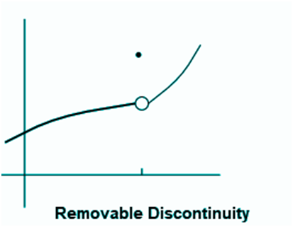
This type of discontinuity can be easily eliminated by redefining the function .
![]()
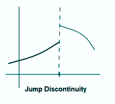
Jump Discontinuity
It is a type of discontinuity, in which the left-hand limit and right-hand limit for a function x = a exists, but they are not equal to each other.![]()
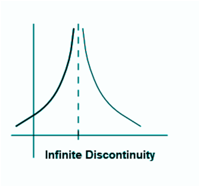
Infinite Discontinuity
The function diverges at x =a to give a discontinuous nature. It means that the function f(a) is not defined. Since the value of the function at x = a does not approach any finite value or tends to infinity, the limit of a function x → a are also not defined.
Example : Discuss the continuity of the function f defined by
f (x) =![]() , x ¹0.
, x ¹0.
Solution Fix any non zero real number c, we have
![]() =
= ![]() =
= ![]() = f( c )
= f( c )
and hence, f is continuous
at every point in the domain of f. Thus f is a continuous function.
Definition -3:
The (ε, δ)-definition of continuity. We recall the definition of continuity: Let f : [a, b] → R and x0 ∈ [a, b]. f is continuous at x0 if for every ε > 0 there exists δ > 0 such that |x − x0| < δ implies |f(x) − f(x![]() )| < ε. We sometimes indicate that the δ may depend on ε by writing δ(ε).
)| < ε. We sometimes indicate that the δ may depend on ε by writing δ(ε).
Example:
The function defined by f (x) = √x is continuous.
Proof:
Given ε > 0 we must show that |√x - √p| < ε provided that x, p are close enough.
Now |√x - √p| = |x - p|/|√x + √p| < |x - p| /√p and so choosing δ = ε/√p will do.
Definition
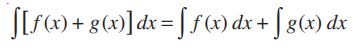
If f and g are functions from R to R, we define the function f + g by (f + g)(x) = f (x) + g(x) for all x in R.
Similarly we may define the difference, product and quotient of functions.
Theorem
If f and g are continuous a point p of R, then so are f + g, f - g, f.g and (provided g(p) ≠ 0) f /g .
Proof
This follows directly from the corresponding arithmetic properties of sequences.
For example: to prove that f + g is continuous at p ∈ R
Suppose (xn)→ p. We are told that (f (xn))→ f (p) and (g(xn))→ g(p) and we must prove that (f + g)(xn))→ (f + g)(p).
But the LHS of this expression is f (xn) + g(xn) and the RHS is f (p) + g(p) and so the result follows from the arithmetic properties of sequences
Theorem
The composite of continuous functions is continuous.
Proof
Suppose f: R→ R and g: R→ R. Then the composition g  f is defined by g f (x) = g(f (x)).
We assume that f is continuous at p and that g is continuous at f (p). So suppose that (xi)→ p. Then (f (xi))→ f (p) and then (g(f (xi)))→ g(f (p)) which is what we need.
Examples
- Clearly the identity function which x ↦ x is continuous.
Hence, using the above, any polynomial function is continuous and hence any rational function (a ratio of polynomial functions) is continuous at any point where the denominator is non-zero. - We will prove later that functions like √x, sinx, cosx, exp(x), logx, ... are continuous. It follows that , for example sin2(x + 5), exp(-x2), √(1 + x4), ... are continuous since they are made by composing continuous functions.
![]()
Hence, the function f(x) is continuous at x =0.
Algebra of continuous functions:
Theorem : Suppose f and g be two real functions continuous at a real number c.
Then
(1) f + g is continuous at x = c.
(2) f – g is continuous at x = c.
(3) f . g is continuous at x = c.
(4) f/g is continuous at x = c, (provided g(c) ¹0).
(5) the algebraic operations between two functions are also continuous.
(6) f(g(x)) and g(f(x)) are continuous at x = a (Composite Function is continuous)
(7) Trigonometric Function is Continuous
(8) Exponential Function is Continuous
(9) Logarithm function is continuous .
(10) Polynomial Function is continuous.
(11) Modulus Function is Continuous.
(12) All rational functions are continuous.
Proof: (1) Given,
limx→a f(x) = f(a)
limx→ a g(x) = g(a)
Now as per the theorem,
limx → a (f+g)(x) ⇒ lim x → c [f(x) + g(x)]
⇒ limx → c f(x) + limx → c g(x)
⇒ f(a) + g(a)
⇒ (f + g)(a)
Therefore,
limx → a (f+g)(x) = (f + g)(c)
Hence, f+g is continuous at x = a.
(3)
Proof: Given,
limx→a f(x) = f(a)
limx→ a g(x) = g(a)
So, the limit of product of two functions, f and g at x is given by:
limx → a (f . g)(x) ⇒ lim x → c [f(x) . g(x)]
⇒ limx → c f(x) . limx → c g(x)
⇒ f(a) . g(a)
⇒ (f . g)(a)
Therefore,
limx → a (f . g)(x) = (f . g)(c)
Hence, f . g is continuous at x = a.
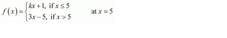
Question :Find the values of k so that the function f is continuous at the indicated point.
ANSWER:
The given function f is
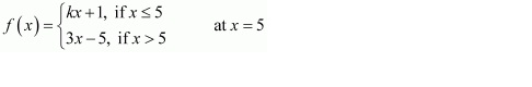
The given function f is continuous at x = 5, if f is defined at x = 5 and if the value of f at x = 5 equals the limit of f at x = 5
It is evident that f is defined at x = 5 and f(5)=kx+1=5k+1
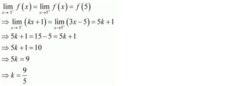
Therefore, the required value of 9/5.
Problem:
Prove that the function defined by f(x) = | cos x | is a continuous function.
Solution: Given, f(x) = |cos x|
f(x) is the real function for all real numbers ‘x’ and the domain of f(x) is the real number
Let g(x) = cos x and h(x) = |x|
g(x) and h(x) are cosine functions and modulus functions are continuous for all real numbers.
Now,
(goh) (x) = g (h(x)) = g(|x|) = cos |x| is a composite function, hence is a continuous function. But it is not equal to f(x).
Again,
(hog) (x) = h(g(x)) = g(cos x) = |cos x| = f(x) [Given]
Hence,
f(x) = |cos x| = hog (x) is a composition function of two continuous functions. Therefore, it is also a continuous function.
Continuity in open interval (a, b)
f(x) will be continuous in the open interval (a,b) if at any point in the given interval the function is continuous.
Continuity in closed interval [a, b]
A function f(x) is said to be continuous in the closed interval [a,b] if it satisfies the following three conditions.
1) f(x) is be continuous in the open interval (a, b)
2) f(x) is continuous at the point a from right i.e.![]()
3) f(x) is continuous at the point b from left i.e. ![]()
1. Study applications of the derivative
- Books Name
- Mathmatics Book Based on NCERT
- Publication
- KRISHNA PUBLICATIONS
- Course
- CBSE Class 12
- Subject
- Mathmatics
Chapter 6
Applications of Derivatives:
Derivatives have various important applications in Mathematics such as
- To find the Rate of Change of a Quantities,
- To find the equation of Tangent and Normal to a Curve, and
- To find turning points on the graph of a function which in turn will help us to locate points at which largest or smallest value (locally) of a function occurs,
- To find intervals on which a function is increasing or decreasing.
- To find the Approximation Value,
- To find the Minimum and Maximum Values of algebraic expressions.
Application of Derivatives in Real Life
- To calculate the profit and loss in business using graphs.
- To check the temperature variation.
- To determine the speed or distance covered such as miles per hour, kilometre per hour etc.
- Derivatives are used to derive many equations in Physics.
- Infinite series representation of functions,
- Optimization problems
1. Concept of Integrals and types of integral
- Books Name
- Mathmatics Book Based on NCERT
- Publication
- KRISHNA PUBLICATIONS
- Course
- CBSE Class 12
- Subject
- Mathmatics
Chaper 7
Integrals
Integration is the act of bringing together smaller components into a single system that functions as one.
Differentiation is the process of finding the derivative of the functions and integration is the process of finding the antiderivative of a function. So, these processes are inverse of each other. So we can say that integration is the inverse process of differentiation or vice versa. The integration is also called the anti-differentiation. In this process, we are provided with the derivative of a function and asked to find out the function (i.e., primitive).
To represent the antiderivative of “f”, the integral symbol “∫” symbol is introduced. The antiderivative of the function is represented as ∫ f(x) dx. This can also be read as the indefinite integral of the function “f” with respect to x.
Therefore, the symbolic representation of the antiderivative of a function (Integration) is:
y = ∫ f(x) dx
y=∫ f(x) dx = F(x) + C.
Types of Integrals
Two types of integrals in maths:
- Definite Integral
- Indefinite Integral
Definite Integral
An integral that contains the upper and lower limits then it is a definite integral. On a real line, x is restricted to lie. Riemann Integral is the other name of the Definite Integral.
A definite Integral is represented as:

Indefinite Integral
Indefinite integrals are defined without upper and lower limits. It is represented as:
∫f(x)dx = F(x) + C
Where C is any constant and the function f(x) is called the integrand.
Properties Indefinite Integral:
1.
2.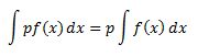 or
or
![]()
3. For a finite number of functions f1, f2…. fn and the real numbers p1, p2…pn,
∫[p1f1(x) + p2f2(x)….+pnfn(x) ]dx = p1∫f1(x)dx + p2∫f2(x)dx + ….. + pn∫fn(x)dx
1. Area under Simple Curves especially lines, circles/ parabolas/ellipses (in standard form only)
- Books Name
- Mathmatics Book Based on NCERT
- Publication
- KRISHNA PUBLICATIONS
- Course
- CBSE Class 12
- Subject
- Mathmatics
Chapter 8
Area under Simple Curves especially lines, circles/ parabolas/ellipses (in standard form
One of the major application of integrals is in determining the area under the curves.
Consider a function y = f(x), then the area is given as
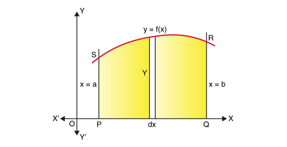
![]()
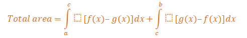
Consider the two curves having equation of f(x) and g(x), the area between the region a,b of the two curves is given as-
dA = f(x) – g(x)]dx, and the total area A can be taken as- 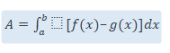
Application of Integrals Examples
Example 1:
Determine the area enclosed by the circle x2 + y2 = a2
Solution:
Given, circle equation is x2 + y2 = a2
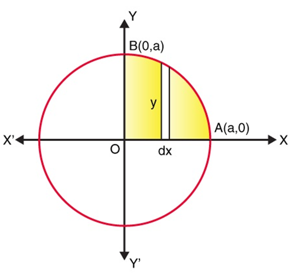
From the given figure, we can say that the whole area enclosed by the given circle is as
= 4(Area of the region AOBA bounded by the curve, coordinates x=0 and x=a, and the x-axis)
As the circle is symmetric about both x-axis and y-axis, the equation can be written as
= 4 0∫a y dx (By taking the vertical strips) ….(1)
From the given circle equation, y can be written as
y = ±√(a2-x2)
As the region, AOBA lies in the first quadrant of the circle, we can take y as positive, so the value of y becomes √(a2-x2)
Now, substitute y = √(a2-x2) in equation (1), we get
= 4 0∫a √(a2-x2) dx
Integrate the above function, we get
= 4 [(x/2)√(a2-x2) +(a2/2)sin-1(x/a)]0 a
Now, substitute the upper and lower limit, we get
= 4[{(a/2)(0)+(a2/2)sin-1 1}-{0}]
= 4(a2/2)(π/2)
= πa2.
Hence, the area enclosed by the circle x2 +y2 =a2 is πa2.
1. Basic Concepts of Differential Equations and Types of Differential equations
- Books Name
- Mathmatics Book Based on NCERT
- Publication
- KRISHNA PUBLICATIONS
- Course
- CBSE Class 12
- Subject
- Mathmatics
Chapter 9
Differential Equations
Basic Concepts of Differential Equations and Types of Differential equations
Differential Equations:
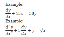
A differential equation is any equation which contains derivatives, either ordinary derivatives or partial derivatives.
Example:
Example:
Differential equation into two types:
- Ordinary differential equation
- partial differential equations.
[1] Ordinary differential equation:
An ordinary differential equation is an equation which is defined for one or more functions of one independent variable and its derivatives. It is abbreviated as ODE.
y'=x+1 is an example of ODE.
An ordinary differential equation is a differential equation that does not involve partial derivatives
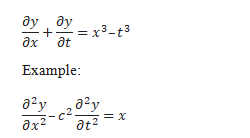
[2] partial differential equations. :
A partial differential equation (or briefly a PDE) is a mathematical equation that involves two or more independent variables, an unknown function (dependent on those variables), and partial derivatives of the unknown function with respect to the independent variables.
A partial differential equation is a differential equation that involves partial derivatives.
Example:
2. Concept of Differentiability and Algebra of derivatives
- Books Name
- Mathmatics Book Based on NCERT
- Publication
- KRISHNA PUBLICATIONS
- Course
- CBSE Class 12
- Subject
- Mathmatics
Concept of Differentiability and Algebra of derivatives :
Differentiability:
A function is differentiable at a point when there's a defined derivative at that point. This means that the slope of the tangent line of the points from the left is approaching the same value as the slope of the tangent of the points from the right.
The computation of the slope of a tangent line, the instantaneous rate of change of a function, and the instantaneous velocity of an object at x=a all required us to compute the following limit.
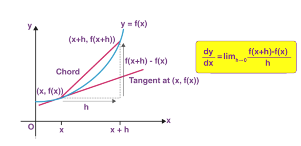
A function f : U -> R, defined on an open set UÍR, is said to be differentiable at aÎU, if the derivative
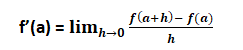
exists. This implies that the function is continuous at a.
This function f is said to be differentiable on U if it is differentiable at every point of U. In this case, the derivative of f is thus a function from U into R.
A continuous function is not necessarily differentiable, but a differentiable function is necessarily continuous (at every point where it is differentiable)
The derivative of f(x) with respect to x is the function f′(x) and is defined as,
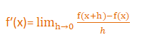
Derivative of f at c is denoted by f ¢(c) or ![]()
![]()
wherever the limit exists is defined to be the derivative of f.
The derivative of f is denoted by f '(x) or ![]()
The process of finding derivative of a function is called differentiation.
Algebra of derivatives:
Properties: Let u=u(x), v=v(x) and w=w(x) be three differentiable function.
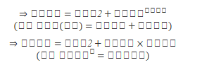
(1) (u ± v)¢ = u¢ ± v (Sum Rule of Differentiation)
(2) (uv)¢ = u¢v + uv¢ (Leibnitz or product rule)
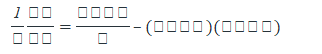
(3)![]() ,wherever v ¹ 0 (Quotient rule).
,wherever v ¹ 0 (Quotient rule).
(4) (uvw)’ = uv w’ + uwv’ + vw u’
Theorem : If a function f is differentiable at a point c, then it is also continuous at that
point.
Solution :
Since f is differentiable at c, we have
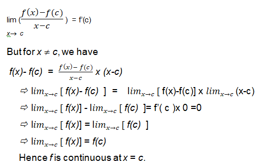
Corollary : Every differentiable function is continuous but vice versa is not true.
we have seen that the function defined by f (x) = | x| is a continuous function.
Consider the
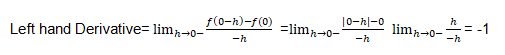
![]()
Since the above left and right hand Derivative at 0 are not equal,
Limit does not exist and hence f is not differentiable at 0.
Thus every continuous function is not differentiable function.
3. Derivatives of composite functions
- Books Name
- Mathmatics Book Based on NCERT
- Publication
- KRISHNA PUBLICATIONS
- Course
- CBSE Class 12
- Subject
- Mathmatics
Derivatives of composite functions
Theorem: (Chain Rule) Let f be a real valued function which is a composite of two
functions u and v; i.e., f = v o u. Suppose t = u(x) and if both 
we have ![]()
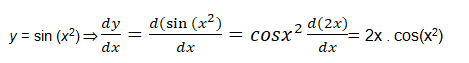
Example: Find the derivative of the function given by f (x) = sin (x2).
Ans:
Let
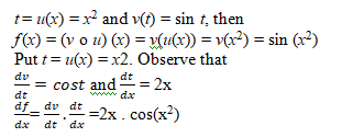
Alternatively, We can also directly proceed as follows:
Example :
Find the derivative of sin x – cos x.
Solution:
Given function is: sin x – cos x
Let f(x) = sin x and g(x) = cos x
Using the difference rule of differentiation,
d/dx [f(x) – g(x)] = d/dx f(x) – d/dx g(x)
d/dx (sin x – cos x) = d/dx (sin x) – d/dx (cos x)
= cos x – (-sin x)
= cos x + sin x
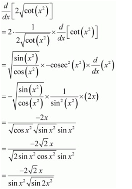
Problem:
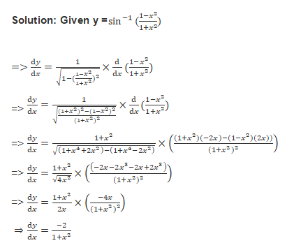
Differentiate the functions with respect to x.
![]()
Ans;
10. Mean Value Theorem
- Books Name
- Mathmatics Book Based on NCERT
- Publication
- KRISHNA PUBLICATIONS
- Course
- CBSE Class 12
- Subject
- Mathmatics
Mean Value Theorem:
Rolle’s Theorem which states that:
Rolle’s Mean Value Theorem
If a function f is defined in the closed interval [a, b] in such a way that it satisfies the following conditions.
i) The function f is continuous on the closed interval [a, b]
ii)The function f is differentiable on the open interval (a, b)
iii) and f (a) = f (b) ,
then there exists at least one value of x=cÎ (a, b) such that f'(c) = 0.
Geometric interpretation of Rolle’s Theorem
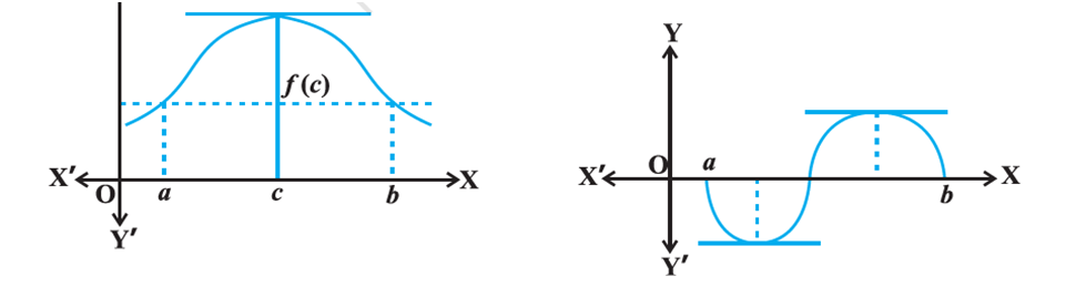
Observe what happens to the slope of the tangent to the curve at various points
between a and b. In each of the graphs, the slope becomes zero at least at one point.
That is precisely the claim of the Rolle’s theorem as the slope of the tangent at any
point on the graph of y = f (x) is nothing but the derivative of f (x) at that point.
Lagrange’s Mean Value Theorem (LMVT)
Lagrange’s Mean Value Theorem or First Mean Value theorem states that a function f is defined in the closed interval [a, b], it satisfies the following conditions:
- The function f is always continuous in the closed interval [a, b]
- The function is always differentiable in the open interval (a, b)
And there exists at least one value x = cÎ (a,b) such that,
[f(b)–f(a)]/ (b-a) = f’ (c)
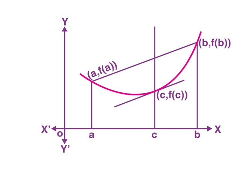
Geometrical Representation of Lagrange’s Mean Value Theorem
The graph given below the curve y = f(x) is The function f is
i) continuous on the closed interval [a, b]
ii)The function f is differentiable on the open interval (a, b)
then, According to the Lagrange Mean Value Theorem,
Any function that is continuous on [a,b] and also differentiable on (a,b) has some in the interval (a,b) such that the secant joining the interval's ends is parallel to the tangent at point C.
f ’(c) = [ f (b) –f (a)]/(b-a)
Example:
Verify Mean Value Theorem for the function f(x) = x2 – 4x – 3 in the interval [a, b], where a = 1 and b = 4.
Solution:
Given,
f(x) = x2 – 4x – 3
f'(x) = 2x – 4
a = 1 and b = 4 (given)
f(a) = f(1) = (1)2 – 4(1) – 3 = 1 – 4 – 3 = -6
f(b) = f(4) = (4)2 – 4(4) – 3 = -3
Now,
[f(b) – f(a)]/ (b – a) = (-3 + 6)/(4 – 1) = 3/3 = 1
As per the Lagrange’s mean value theorem statement, there is a point c ∈ (1, 4) such that
f'(c) = [f(b) – f(a)]/ (b – a),
i.e. f'(c) = 1.
2c – 4 = 1
2c = 5
c = 5/2 ∈ (1, 4)
Verification: f'(c) = 2(5/2) – 4 = 5 – 4 = 1
Hence, verified the mean value theorem.
Example:
Verify Rolle’s theorem for the function y = x2 + 2, a = –2 and b = 2.
Solution:
From the definition of Rolle’s theorem, the function y = x2 + 2 is continuous in [– 2, 2] and differentiable in (– 2, 2).
From the given,
f(x) = x2 + 2
f(-2) = (-2)2 + 2 = 4 + 2 = 6
f(2) = (2)2 + 2 = 4 + 2= 6
Thus, f(– 2) = f( 2) = 6
Hence, the value of f(x) at –2 and 2 coincide.
Now, f'(x) = 2x
Rolle’s theorem states that there is a point c ∈ (– 2, 2) such that f′(c) = 0.
At c = 0, f′(c) = 2(0) = 0, where c = 0 ∈ (– 2, 2)
Hence verified.
4. Derivatives of implicit functions
- Books Name
- Mathmatics Book Based on NCERT
- Publication
- KRISHNA PUBLICATIONS
- Course
- CBSE Class 12
- Subject
- Mathmatics
Derivatives of implicit functions:
Implicit functions are functions where a specific variable cannot be expressed as a function of the other variable. A function that depends on more than one variable.
we’ll adopt the following procedure:
- Given an implicit function with the dependent variable y and the independent variable x (or the other way around).
- Differentiate the entire equation with respect to the independent variable (it could be x or y).
- After differentiating, we need to apply the chain rule of differentiation.
- Solve the resultant equation for dy/dx (or dx/dy likewise) or differentiate again if the higher-order derivatives are needed.
“Some function of y and x equals to something else”. Knowing x does not help us compute y directly.
Example, x2 + y2 = r2 (Implicit function)
Differentiate with respect to x:
d(x2) /dx + d(y2)/ dx = d(r2) / dx
Solve each term:
Using Power Rule: d(x2) / dx = 2x
Using Chain Rule : d(y2)/ dx = 2y dydx
r2 is a constant, so its derivative is 0: d(r2)/ dx = 0
Which gives us:
2x + 2y dy/dx = 0
Collect all the dy/dx on one side
y dy/dx = −x
Solve for dy/dx:
dy/dx = −xy
Example . Find dy/dx if x2y3 − xy = 10.
Solution:
2xy3 + x2. 3y2 . dy/dx – y – x . dy/dx = 0
(3x2y2 – x ) . dy/dx = y – 2xy3
dy/dx = (y – 2xy3) / (3x2y2 – x)
Example . Find dy/dx if y = sinx + cosy
Solution:
y – cosy = sinx
dy/dx + siny. dy/dx = cosx
dy/dx = cosx / (1 + siny)
Example . Find the slope of the tangent line to the curve x2+ y2= 25 at the point (3,−4).
Solution:
Note that the slope of the tangent line to a curve is the derivative, differentiate implicitly with respect to x, which yields,
2x + 2y. dy/dx = 0
dy/dx = -x/y
Hence, at (3,−4), y′ = −3/−4 = 3/4, and the tangent line has slope 3/4 at the point (3,−4).
5. Derivatives of inverse trigonometric functions
- Books Name
- Mathmatics Book Based on NCERT
- Publication
- KRISHNA PUBLICATIONS
- Course
- CBSE Class 12
- Subject
- Mathmatics
Derivatives of inverse trigonometric functions:
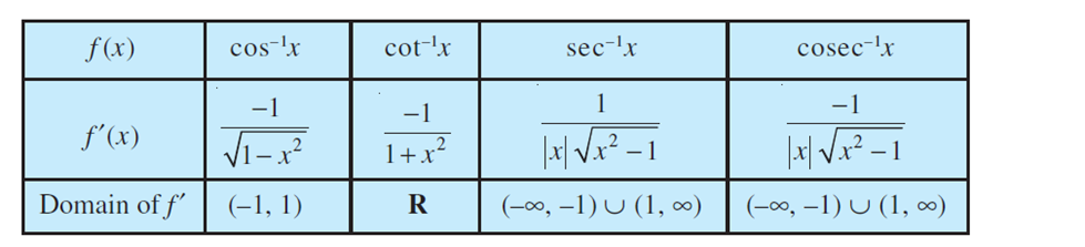
Inverse of sin x = arcsin(x) or
Let us now find the derivative of Inverse trigonometric function
Example: Find the derivative of a function ![]()
Solution: Given
![]()
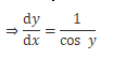
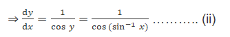
Differentiating the above equation w.r.t. x, we have:
Putting the value of y form (i), we get
From equation (ii), we can see that the value of cos y cannot be equal to 0, as the function would become undefined ![]()
i. e.![]()
From (i) we have ![]()
![]()
Using property of trigonometric function,
![]()
![]()
Now putting the value of (iii) in (ii), we have ![]()
Therefore, the Derivative of Inverse sine function is ![]()
Example:Find the derivative of a function
Problem: y = cot-1(1/x2)
Solution:
As we are solving the above three problem in the same way this problem will solve
By using chain rule,
y’ = (cot-1(1 / x2))’
= { – 1 / (1 + (1 / x2))2 } . (1 / x2)’
= { – 1 / (1 + (1 / x4)) . (-2x-3)
= 2x4 / (x4 + 1)x3
Example: Solve f(x) = tan-1(x) Using first Principle.
Solution:
For solving and finding tan-1x, we have to remember some formulae, listed below.
- limh->0 {f(x + h) – f(x)} / h
- tan-1(θ/θ) = 1
- tan-1x – tan-1y = tan-1[(x – y) / (1 + xy)]
f(x) = tan-1x
f(x + h) = tan-1(x + h)
Apply 1st formula
limh->0 {tan-1(x + h) – tan-1x } / h
Now Apply 3rd formula
limh->0 tan-1[(x – h – x) / (1 + (x + h)x] / h
limh->0 tan-1[(h / (1 + x2 + xh ] / h . [(1 + x2 + xh) / (1 + x2 + xh)]
limh->0 tan-1 {h / 1 + x2 + xh} / {h / 1 + x2 + xh} . limh->0 1 / 1 + x2 + xh
Now we made the solution like so that we apply the 2nd formula
= 1 . 1 / (1 + x2 + x . 0)
= 1 / (1 + x2)
6. Derivatives of Exponential and Logarithmic Functions
- Books Name
- Mathmatics Book Based on NCERT
- Publication
- KRISHNA PUBLICATIONS
- Course
- CBSE Class 12
- Subject
- Mathmatics
Derivatives of Exponential and Logarithmic Functions:
7. Logarithmic Differentiation
- Books Name
- Mathmatics Book Based on NCERT
- Publication
- KRISHNA PUBLICATIONS
- Course
- CBSE Class 12
- Subject
- Mathmatics
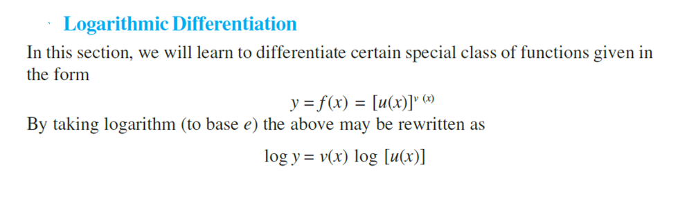
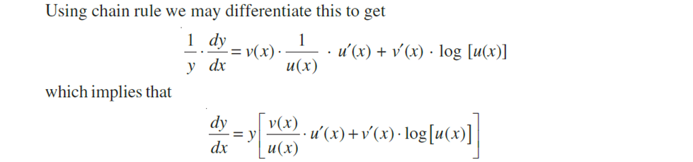
Logarithmic Differentiation:
If function to the power function or function to the power variable or variable to the power function or variable to the power variable ,then apply logarithm.
The derivative of ex w.r.t. x = d/dx (ex) = ex
The derivative of log x w.r.t. x = d/dx (log x) = 1/x
Now this last limit  is exactly the definition of above derivative f'(x) at x = 0, i.e f'(0). Therefore, the derivative becomes,
f'(x) = bxf'(0) = bx
So, in case of natural exponential functions, f(x) = ex
Note: In general exponential cases, for example, y = bx, where b is a real number. The derivative for this kind of function is
![]()
Question: Differentiate f(x) = 4ex – 5x
Answer:
The derivation of ex will remain ex, the derivative of 5x will become 5xln(5) as explained above.
Therefore, f'(x) = 4ex – 5xln(x)
Question : Find the value of F'(x) at x=0 when f(x) = 7x + 2ex
Answer:
Differentiating: f'(x) = 7xln(7) + 2ex
at x=0, f'(0) = 70ln(7) + 2e0
= ln(7) + 2
= 3.945
Question: d/dx(xx) = xx(1+ln x)
Question: Find the value of
if y = 2x{cos x}.
Solution: Given the function y = 2x{cos x}
Taking logarithm of both the sides, we get
log y = log(2x{cos x})
Now, differentiating both the sides w.r.t by using the chain rule we get,
8. Derivatives of Functions in Parametric Forms
- Books Name
- Mathmatics Book Based on NCERT
- Publication
- KRISHNA PUBLICATIONS
- Course
- CBSE Class 12
- Subject
- Mathmatics
Derivatives of Functions in Parametric Forms:
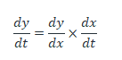
A parametric derivative is a derivative of a dependent variable with respect to another dependent variable that is taken when both variables depend on an independent third variable, usually thought of as "time" (that is, when the dependent variables are x and y and are given by parametric equations in t).
More precisely, a relation expressed between two variables x and y in the form
x = f (t), y = g(t) is said to be parametric form with t as a parameter.
or

This is the required solution.
9. Second Order Derivative
- Books Name
- Mathmatics Book Based on NCERT
- Publication
- KRISHNA PUBLICATIONS
- Course
- CBSE Class 12
- Subject
- Mathmatics
Second Order Derivative:
The first-order derivative at a given point gives us the information about the slope of the tangent at that point or the instantaneous rate of change of a function at that point. Second-Order Derivative gives us the idea of the shape of the graph of a given function. The second derivative of a function f(x) is usually denoted as f”(x). It is also denoted by D2y or y2 or y” if y = f(x).
Let y = f(x)
Then, dy/dx = f'(x)
If f'(x) is differentiable, we may differentiate (1) again w.r.t x. Then, the left-hand side becomes d/dx(dy/dx) which is called the second order derivative of y w.r.t x.
Example: Find d2y/dx2, if y = x3?
Solution:
Given that, y = x3
Then, first derivative will be
dy/dx = d/dx (x3) = 3x2
Again, we will differentiate further to find its
second derivative,
Therefore, d2y/dx2 = d/dx (dy/dx)
= d/dx (3x2)
= 6x
Example : Find d2y/dx2, if y = Asinx + Bcosx, Where A and B are constants?
Solution:
Given that, y = Asinx + Bcosx
Then, first derivative will be
dy/dx = d/dx (Asinx + Bcosx)
= A d/dx (sinx) + B d/dx (cosx)
= A(cosx) + B(-sinx)
= Acosx – Bsinx
Again, we will differentiate further to find its second derivative,
d2y/dx2 = d/dx (dy/dx)
= d/dx (Acosx – Bsinx)
= A d/dx (cosx) – B d/dx (sinx)
= A(-sinx) – B(cosx)
= -Asinx – Bcosx
= -(Asinx + Bcosx)
= -y
Example: If x = t + cost, y = sint, find the second derivative.
Solution:
Given that, x = t + cost and y = sint
First Derivative,
dy/dx = (dy/dt) / (dx/dt)
= (d/dt (sint)) / (d/dt (t + cost))
= (cost) / (1 – sint) ……. (1)
Second Derivative,
d2y / dx2 = d/dx (dy/dx)
= d/dx (cost / 1 – sint) …….. (from eq.(1))
= d/dt (cost / 1 – sint) / (dx/dt) ………(chain rule)
= ((1 – sint) (-sint) – cost(-cost)) / (1 – sint)2 / (dx/dt) …. (quotient rule)
= (-sint + sin2t + cos2t) / (1 – sint)2 / (1 – sint)
= (-sint + 1) / (1 – sint)3
= 1 / (1 – sint)2
2. Rate of Change of Quantities
- Books Name
- Mathmatics Book Based on NCERT
- Publication
- KRISHNA PUBLICATIONS
- Course
- CBSE Class 12
- Subject
- Mathmatics
Rate of Change of Quantities :
![]() , we mean the rate of change of distance s with respect to the time t.
, we mean the rate of change of distance s with respect to the time t.
![]() the rate of change of y with respect to x.= f′ (x)
the rate of change of y with respect to x.= f′ (x)
![]() x=x0 (or f′ (x0 )) represents the rate of change
x=x0 (or f′ (x0 )) represents the rate of change
Further, if two variables x and y are varying with respect to another variable t, i.e., if x= f( t) and y =g (t), then by Chain Rule.
![]() ,if
,if ![]()
Thus, the rate of change of y with respect to x can be calculated using the rate of change of y and that of x both with respect to t.
Example :
Find the rate of change of the area of a circle per second with respect to its radius r when r = 5 cm
Answer:
The area A of a circle with radius r is given by A = π r 2 . Therefore, the rate of change of the area A with respect to its radius r is given by ![]()
When r = 5 cm. ![]()
Thus, the area of the circle is changing at the rate of 10π cm2 /s.
Example :
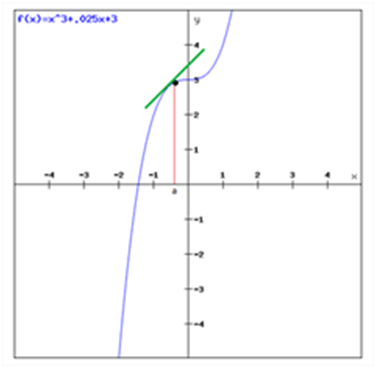
The volume of a cube is increasing at a rate of 9 cubic centimetres per second. How fast is the surface area increasing when the length of an edge is 10 centimetres ?
Solution:
Let x be the length of a side, V be the volume and S be the surface area of the cube. Then, V = x 3 and S = 6x 2 , where x is a function of time t. Now
Example : The total cost C(x) in Rupees, associated with the production of x units of an item is given by C(x) = 0.005 x 3 – 0.02 x 2 + 30x + 5000
Find the marginal cost when 3 units are produced, where by marginal cost we mean the instantaneous rate of change of total cost at any level of output.
Solution: Since marginal cost is the rate of change of total cost with respect to the output, we have Marginal cost (MC) =![]() = 0.005(3x2) - 0.02(2x ) + 30
= 0.005(3x2) - 0.02(2x ) + 30
When x = 3, MC = 0.015(32)- 0.04(3) + 30 = 0.135 – 0.12 + 30 = 30.015.
Hence, the required marginal cost is ` 30.02 (nearly).
3. Increasing and Decreasing Functions
- Books Name
- Mathmatics Book Based on NCERT
- Publication
- KRISHNA PUBLICATIONS
- Course
- CBSE Class 12
- Subject
- Mathmatics
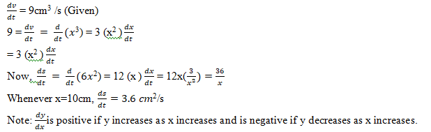
Increasing and Decreasing Functions:
Definition : Let I be an interval contained in the domain of a real valued function f.
Then f is said to be
- increasing on I if x1 < x2 in I ⇒f(x1 ) < f(x2 ) for all x1 , x2 ∈ I.
(ii) decreasing on I, if x 1 , x 2 in I ⇒f(x 1 ) < f(x 2 ) for all x 1 , x 2 ∈ I.
- constant on I, if f(x) = c for all x ∈ I, where c is a constant.
(iv) decreasing on I if x1 < x2 in I ⇒ f (x1 ) ≥ f(x2 ) for all x1 , x2 ∈ I.
- strictly decreasing on I if x1 < x2 in I ⇒ f(x1 ) > f(x2 ) for all x1 , x2 ∈ I.
Definition :
Let x 0 be a point in the domain of definition of a real valued function f. Then f is said to be increasing, decreasing at x0 if there exists an open interval I containing x 0 such that f is increasing, decreasing, respectively, in I
Example :
Show that the function given by f(x) = 7x – 3 is increasing on R.
Solution:
Let x1 and x Î R. Then x1 < x2 ⇒ 7x1 < 7x2 ⇒ 7x1 – 3 < 7x2 – 3 ⇒ f(x1 ) < f(x2 ) Thus, by Definition ,
it follows that f is strictly increasing on R.
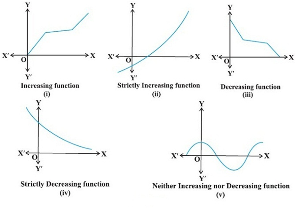
Theorem 1 :
Let f be continuous on [a, b] and differentiable on the open interval (a,b).
Then (a) f is increasing in [a,b] if f ′(x) > 0 for each x ∈ (a, b)
(b) f is decreasing in [a,b] if f ′(x) < 0 for each x ∈ (a, b)
(c) f is a constant function in [a,b] if f ′(x) = 0 for each x ∈ (a, b)
Proof :
- Let x1 , x2 ∈ [a, b] be such that x1 < x2 . Then, by Mean Value Theorem ,
there exists a point c between x1 and x2
such that f(x2 ) – f(x1 ) = f ′(c) (x2 – x1 )
i.e. f(x2 ) – f(x1 ) > 0 (as f ′(c) > 0 (given))
i.e. f(x2 ) > f(x1 )
Thus, we have x1< x2 =>f (x1 )<f (x2 ), for all x1,x2Î [ a,b ]
Hence, f is an increasing function in [a,b].
The proofs of part (b) and (c) are similar
Example :
Find the intervals in which the function f given by f(x) = x 2 – 4x + 6 is
- increasing (b) decreasing
Solution :
We have f (x) = x 2 – 4x + 6
or f ′(x) = 2x – 4
Therefore, f ′(x) = 0 gives x = 2.
Now the point x = 2 divides the real line into two disjoint intervals namely, (– ∞, 2) and (2, ∞)
In the interval (– ∞, 2), f ′(x) = 2x – 4 < 0.
Therefore, f is decreasing in this interval. Also, in the interval (2, ∞) , f ′(x )> 0
and so the function f is increasing in this interval.
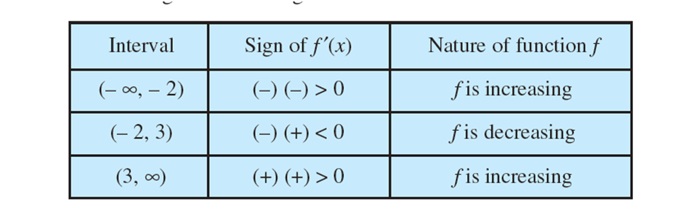
Example :
Find the intervals in which the function f given by f (x) = 4x 3 – 6x 2 – 72x + 30 is
- increasing (b) decreasing.
Solution: We have f(x) = 4x 3 – 6x 2 – 72x + 30
or f ′(x) = 12x 2 – 12x – 72
= 12(x 2 – x – 6) = 12(x – 3) (x + 2)
Therefore, f ′(x) = 0 gives x = – 2, 3.
The points x = – 2 and x = 3 divides the real line into three disjoint intervals, namely,
(– ∞, – 2), (– 2, 3)
and (3, ∞).
In the intervals (– ∞, – 2) and (3, ∞), f ′(x) is positive while in the interval (– 2, 3), f ′(x) is negative. Consequently, the function f is increasing in the intervals (– ∞, – 2) and (3, ∞) while the function is decreasing in the interval (– 2, 3).
However, f is neither increasing nor decreasing in R.
4. Tangents and Normals
- Books Name
- Mathmatics Book Based on NCERT
- Publication
- KRISHNA PUBLICATIONS
- Course
- CBSE Class 12
- Subject
- Mathmatics
Tangents and Normals:
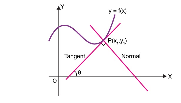
The equation of a straight line passing through a given point (x 1 , y1 ) having finite slope m is given by
y – y1 = m (x – x1 )
The slope of the tangent to the curve y = f(x) at the point (x1 , y1 ) is given by
![]()
So the equation of the tangent at (x1 , y1 ) to the curve y = f (x) is given by
y – y0 = f ′(x1 )(x – x1 )
Note: If a tangent line to the curve y = f (x) makes an angle θ with x-axis in the positive direction, then slope of the tangent =dy/ dx = tan θ .
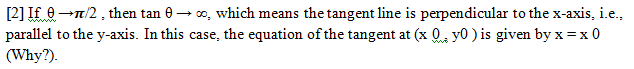
Particular cases:
[1] If slope of the tangent line is zero, then tan θ = 0 and so θ = 0 which means the tangent line is parallel to the x-axis. In this case, the equation of the tangent at the point (x0 , y0 ) is given by y = y0 .
Example ;
Find the slope of the tangent to the curve y = x 3 – x at x = 2.
Solution :
The slope of the tangent at x = 2 is given by ![]()
5. Approximations
- Books Name
- Mathmatics Book Based on NCERT
- Publication
- KRISHNA PUBLICATIONS
- Course
- CBSE Class 12
- Subject
- Mathmatics
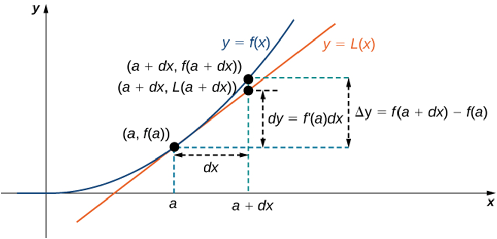
Approximations:
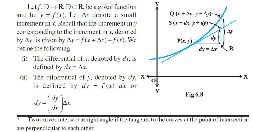
To find a very small change or variation of a quantity, we can use derivatives to give the approximate value of it. The approximate value is represented by delta △.
Suppose change in the value of x, dx = x then,
dy/dx = △x = x.
Since the change in x, dx ≈ x therefore, dy ≈ y.
Example :
Approximate ![]()
using differential.
Solution:
Let us consider y =![]()
, where x = 25 and ∆x = 0.5. Then,
∆y = f(x+∆x) - f(x)=![]()
- ∆y =

- ∆y =

Since dy is approximately equal to ∆y, therefore
![]()
Therefore, the approximate value of ![]()
Example :
Find the approximate value of the function f(3.02), where f(x) is given as 3x2+5x+3.
Solution:
Given that, f(x) = 3x2+5x+3
Assume x = 3, and ∆x = 0.02.
Hence, we can write the given function as:
f (3. 02) = f (x + ∆x) = 3(x + ∆x)2 + 5(x + ∆x) + 3
We know that,
∆y = f (x + ∆x) – f (x).
The above expression can be written as
f (x + ∆x) = f (x) + ∆y
As, dx = ∆x, it can be approximately written as f (x) + f ′(x) ∆x
Hence, f (3.02) ≈ (3x2 + 5x + 3) + (6x + 5) ∆x
Now, substitute the values of x and ∆x, we get
= (3(3)2 + 5(3) + 3) + (6(3) + 5) (0.02)
Now, simplify it to get the approximate value
= (27 + 15 + 3) + (18 + 5) (0.02)
= 45 + 0.46
= 45.46
Therefore, the approximate value of f(3.02) is 45.46.
6. Maxima and Minima
- Books Name
- Mathmatics Book Based on NCERT
- Publication
- KRISHNA PUBLICATIONS
- Course
- CBSE Class 12
- Subject
- Mathmatics
Maxima and Minima
Let x1,x2 ∈ D f(a) > f(x1) and f(a) > f(x2)
A function is said to have a maximum value at a point 'x=a' in its domain D if f(a) ≥ f(x), ∀x ∈ D.
f(a) is called the maximum value of f. "x=a" is called the point of maximum value of f.
Let x1,x2 ∈ D f(a) < f(x1) and f(a) < f(x2)
A function is said to have a minimum value at a point 'a' in its domain D if f(a) ≤ f(x), ∀x ∈ D.
f(a) is called the minimum value of f. "x=a" is called the point of minimum value of f.
Extreme value of function f:
Function f(x) is said to have an extreme value in its domain D if there exists a point a ∈ D such
that f (a) is either the maximum value or the minimum value of f in D.
The number f (a) is called an extreme value of f in D, and point 'a' is called an extreme point.
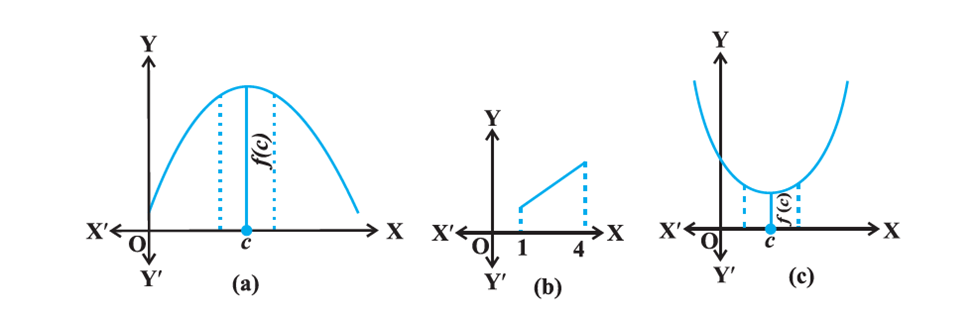
Consider f(x) = 2x2 ,∀ x ∈ R
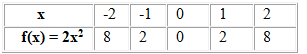
The ordered pairs are (-2,8),(-1,2),(0,0),(1,2) and (2,8).
From the graph, we have f(x) = 0 if x = 0 and f(x) ≥ 0 ∀x ∈ R
The minimum value of f is 0, and the point of minimum value of f is x = 0.
From the graph of the function, f has no maximum value, and hence, no point of maximum value of f in R.
Suppose the domain of f is restricted to [- 2, 1].
The maximum value of the function, f(-2) = 2(-2)2 = 8, which is at x = -2
Note: A function has an extreme value at a point even if it is not differentiable at that point.
Every monotonic function assumes its maximum/minimum value at the end points of the domain of definition of the function.
A more general result is
Every continuous function on a closed interval has a maximum and a minimum
value.
N.B.: Every increasing or decreasing function assumes its maximum or minimum value at the end points of the domain of definition of the function.
Or
Every continuous function on a closed interval has a maximum and a minimum value.
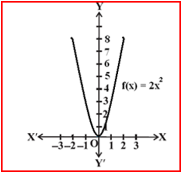
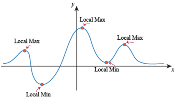
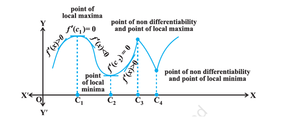
Similarly, the function has maximum value in some neighbourhood of points B and D which are at the top of their respective hills. For this reason, the points A and C may be regarded as points of local minimum value (or relative minimum value) and points B and D may be regarded as points of local maximum value (or relative maximum value) for the function. The local maximum value and local minimum value of the function are referred to as local maxima and local minima, respectively, of the function.
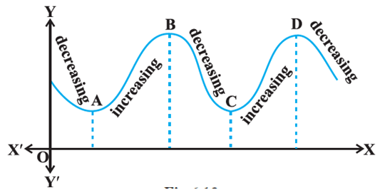
The graph of the function has minimum values in some neighbourhood(nbd) of points Q and S, and has maximum values in some neighbourhood(nbd) of points P, R and T.
The x-coordinates of points P, R and T are called the points of local maximum, and the y-coordinates of points P, R and T, are the local maximum values of f(x).
Similarly, the x-coordinates of points Q and S are called the points of local minimum, and the y-coordinates of points Q and S, are called the local minimum values of f(x).
The local maximum value of a function is said to be the local maxima of that function.
The local minimum value of a function is said to be the local minima of that function.
- When x = a, if f(x) ≤ f(a) for every x in the domain, then f(x) has an Absolute Maximum value and the point a is the point of the maximum value of f.
- When x = a, if f(x) ≤ f(a) for every x in some open interval (p, q) then f(x) has a Relative Maximum value.
- When x= a, if f(x) ≥ f(a) for every x in the domain then f(x) has an Absolute Minimum value and the point a is the point of the minimum value of f.
- When x = a, if f(x) ≥ f(a) for every x in some open interval (p, q) then f(x) has a Relative Minimum value.
Let the point of local maximum value of f in the graph be x = a. The function f is increasing in
the interval (a - h, a) and decreasing in the interval (a , a+h ), where h > 0.
Definition : Let f be a real valued function and let c be an interior point in the domain
of f. Then
(a) c is called a point of local maxima if there is an h > 0 such that
f (c) f (x), for all x in (c – h, c + h), x c
The value f (c) is called the local maximum value of f.
(b) c is called a point of local minima if there is an h > 0 such that
f (c) f (x), for all x in (c – h, c + h)
The value f (c) is called the local minimum value of f .
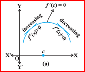
Geometrically, the above definition states that if x = c is a point of local maxima of f,
then the graph of f around c will be as shown in Fig 6.14(a). Note that the function f is
increasing (i.e., f (x) > 0) in the interval (c – h, c) and decreasing (i.e., f (x) < 0) in the
interval (c, c + h).
This suggests that f (c) must be zero.
If f is increasing, then f '(x) > 0, and if f is decreasing, then f '(x) < 0.
If f is neither decreasing nor increasing, then f '(x) = 0. i.e. f '(a) = 0.
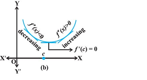
Let the point of local minimum value of f in the graph be x = a.
Function f is decreasing in the interval (a - h, a) and increasing in the interval (a , a+h ), where h > 0. we have f '(a) = 0
Monotonicity
Functions are said to be monotonic if they are either increasing or decreasing in their entire domain. f(x) = ex, f(x) = nx, f(x) = 2x + 3 are some examples.
Functions which are increasing and decreasing in their domain are said to be non-monotonic
For example: f(x) = sin x , f(x) = x2
Monotonicity Of A function At A Point
A function is said to be monotonically decreasing at x = a if f(x) satisfy;
f(x + h) < f(a) for a small positive h
- f'(x) will be positive if the function is increasing
- f'(x) will be negative if the function is decreasing
- f'(x) will be zero when the function is at its maxima or minima
Theorem:
Let f be a real valued function defined on an open interval I. Suppose point a is any arbitrary point in I. If f has a local maxima or a local minima at x = a, then either f '(a) = 0, or f is not differentiable at a.
However, the converse need not be true, i.e. a point at which the derivative vanishes need not be the point of local maxima or local minima.
Every continuous function on a closed interval has a maximum and a minimum value.
Point of Inflection:
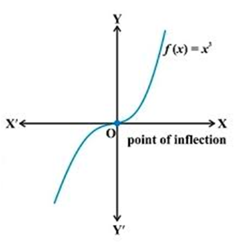
For continuous function f(x), if f'(x0) = 0 or f’”(x0) does not exist at points where f'(x0) exists and if f”(x) changes sign when passing through x = x0 then x0 is called the point of inflection.
(a) If f”(x) < 0, x ∈ (a, b) then the curve y = f(x) in concave downward
(b) if f” (x) > 0, x ∈ (a, b) then the curve y = f(x) is concave upwards in (a, b)
For example: f(x) = sin x
Solution: f'(x) = cos x
f”(x) = sinx = 0 x = nπ, n ∈ z
Critical point:
A point c in the domain of a function f at which either f (c) = 0 or f is not
differentiable is called a critical point of f.
Theorem (First Derivative Test) : Let f be a function defined on an open interval I.
Let f be continuous at a critical point c in I. Then
(i) If f (x) changes sign from positive to negative as x increases through c, i.e., if f (x) > 0 at every point sufficiently close to and to the left of c, and f (x) < 0 at every point sufficiently close to and to the right of c, then c is a point of local maxima.
(ii) If f (x) changes sign from negative to positive as x increases through c, i.e., if f (x) < 0 at every point sufficiently close to and to the left of c, and f (x) > 0 at every point sufficiently close to and to the right of c, then c is a point of local minima.
(iii) If f (x) does not change sign as x increases through c, then c is neither a point of local maxima nor a point of local minima. Infact, such a point is called point of inflection .
Example : Find all points of local maxima and local minima of the function f
given by
f (x) = x3 – 3x + 3.
Solution We have
f (x) = x3 – 3x + 3.
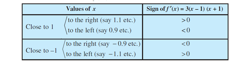
or f (x) = 3x2 – 3 = 3(x – 1) (x + 1)
or f (x) = 0 at x = 1 and x = – 1
Thus, x = ± 1 are the only critical points which could possibly be the points of local
maxima and/or local minima of f . Let us first examine the point x = 1.
Example ; Find all the points of local maxima and local minima of the function f
given by
f (x) = 2x3 – 6x2 + 6x +5.
Solution We have
f (x) = 2x3 – 6x2 + 6x + 5
or f (x) = 6x2 – 12x + 6 = 6(x – 1)2
or f (x) = 0 at x = 1
Thus, x = 1 is the only critical point of f . We shall now examine this point for local maxima and/or local minima of f. Observe that f (x) 0, for all x R and in particular f (x) > 0, for values close to 1 and to the left and to the right of 1. Therefore, by first derivative test, the point x = 1 is neither a point of local maxima nor a point of local minima. Hence x = 1 is a point of inflexion.
Theorem (Second Derivative Test): Let f be a function defined on an interval I and c I. Let f be twice differentiable at c. Then
(i) x = c is a point of local maxima if f (c) = 0 and f (c) < 0 The value f (c) is local maximum value of f .
(ii) x = c is a point of local minima if f (c) 0 and f (c) > 0 In this case, f (c) is local minimum value of f .
(iii) The test fails if f (c) = 0 and f (c) = 0. In this case, we go back to the first derivative test and find whether c is a point of local maxima, local minima or a point of inflexion.
Example : Find local maximum and local minimum values of the function f given by
f (x) = 3x4 + 4x3 – 12x2 + 12
Solution We have
f (x) = 3x4 + 4x3 – 12x2 + 12
or f (x) = 12x3 + 12x2 – 24x = 12x (x – 1) (x + 2)
or f (x) = 0 at x = 0, x = 1 and x = – 2.
Now f (x) = 36x2 + 24x – 24 = 12(3x2 + 2x – 2)
f ‘’(0)=-24 <0
f ‘’(1)= 36 >0
f ‘’(-2)= 72 >0
Therefore, by second derivative test, x = 0 is a point of local maxima and local maximum value of f at x = 0 is f (0) = 12 while x = 1 and x = – 2 are the points of local minima and local minimum values of f at x = – 1 and – 2 are f (1) = 7 and f (–2) = –20, respectively.
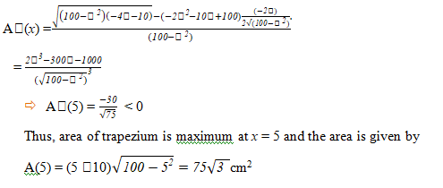
Example : If length of three sides of a trapezium other than base are equal to 10cm, then find the area of the trapezium when it is maximum.
Solution The required trapezium is as given in Figure 6.19.
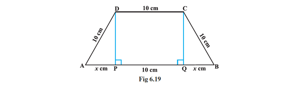
Draw perpendiculars DP and
CQ on AB. Let AP = x cm. Note that APD ~ BQC. Therefore, QB = x cm. Also, by
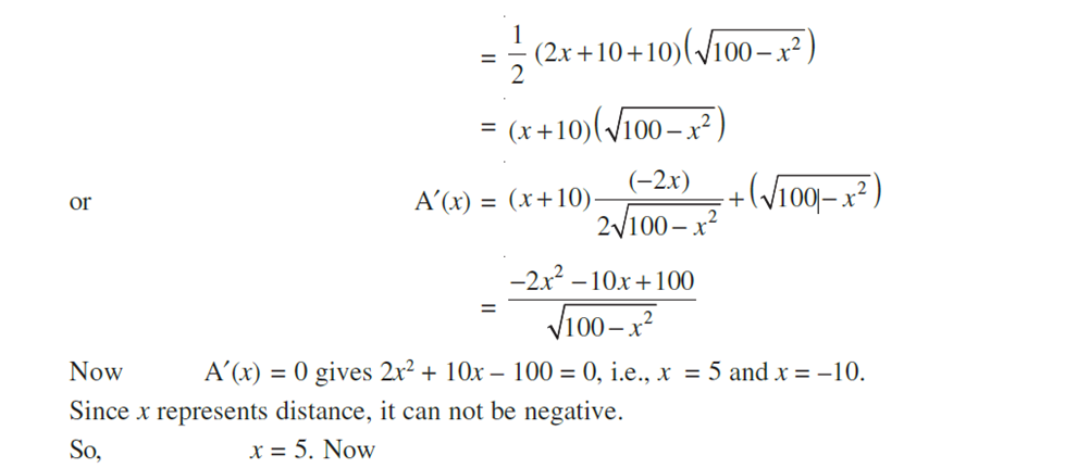
Pythagoras theorem, DP = QC = ![]() . Let A be the area of the trapezium. Then
. Let A be the area of the trapezium. Then
AA(x) = ![]() (sum of parallel sides) (height)
(sum of parallel sides) (height)
Theorem: Let f be a continuous function on an interval I = [a, b]. Then f has the
absolute maximum value and f attains it at least once in I. Also, f has the absolute
minimum value and attains it at least once in I.
Theorem: Let f be a differentiable function on a closed interval I and let c be any
interior point of I. Then
(i) f (c) = 0 if f attains its absolute maximum value at c.
(ii) f (c) = 0 if f attains its absolute minimum value at c.
In view of the above results, we have the following working rule for finding absolute maximum and/or absolute minimum values of a function in a given closed interval [a, b].
Working Rule
Step 1: Find all critical points of f in the interval, i.e., find points x where either f (x) 0 or f is not differentiable.
Step 2: Take the end points of the interval.
Step 3: At all these points (listed in Step 1 and 2), calculate the values of f .
Step 4: Identify the maximum and minimum values of f out of the values calculated in
Step 3: This maximum value will be the absolute maximum (greatest) value of f and the minimum value will be the absolute minimum (least) value of f .
Example: Find the absolute maximum and minimum values of a function f given by
f (x) = 2x3 – 15x2 + 36x +1 on the interval [1, 5].
Solution We have f (x) = 2x3 – 15x2 + 36x +1
or f (x) = 6x2 – 30x + 36 = 6(x – 3) (x – 2)
Note that f (x) = 0 gives x = 2 and x = 3.
We shall now evaluate the value of f at these points and at the end points of the
interval [1, 5], i.e., at x = 1, x = 2, x = 3 and at x = 5. So
f (1) = 2(13) – 15(12) + 36(1) + 1 = 24
f (2) = 2(23) – 15(22) + 36(2) + 1 = 29
f (3) = 2(33) – 15(32) + 36(3) + 1 = 28
f (5) = 2(53) – 15(52) + 36(5) + 1 = 56
Thus, we conclude that absolute maximum value of f on [1, 5] is 56, occurring at x =5, and absolute minimum value of f on [1, 5] is 24 which occurs at x = 1.
2. Integration as an Inverse Process of Differentiation
- Books Name
- Mathmatics Book Based on NCERT
- Publication
- KRISHNA PUBLICATIONS
- Course
- CBSE Class 12
- Subject
- Mathmatics
Integration as an Inverse Process of Differentiation
Example : Find the anti derivative F of f defined by f (x) = 4x3 – 6, where F (0) = 3
Solution: One anti derivative of f (x) is x4 – 6x since
![]()
Therefore, the anti derivative F is given by
F(x) = x4 – 6x + C, where C is constant.
Given that F(0) = 3, which gives,
3 = 0 – 6 0 + C or C = 3
Hence, the required anti derivative is the unique function F defined by
F(x) = x4 – 6x + 3.
3. Geometrical interpretation and Some properties of indefinite integral
- Books Name
- Mathmatics Book Based on NCERT
- Publication
- KRISHNA PUBLICATIONS
- Course
- CBSE Class 12
- Subject
- Mathmatics
Geometrical interpretation and Some properties of indefinite integral
Comparison between differentiation and integration
1. Both are operations on functions.
2. Both satisfy the property of linearity, i.e.,
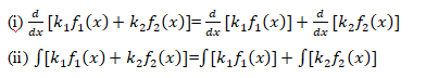
Here k1 and k2 are constants.
3. We have already seen that all functions are not differentiable. Similarly, all functions
are not integrable. We will learn more about nondifferentiable functions and
nonintegrable functions in higher classes.
4. The derivative of a function, when it exists, is a unique function. The integral of
a function is not so. However, they are unique upto an additive constant, i.e., any
two integrals of a function differ by a constant.
5. When a polynomial function P is differentiated, the result is a polynomial whose
degree is 1 less than the degree of P. When a polynomial function P is integrated,
the result is a polynomial whose degree is 1 more than that of P.
6. We can speak of the derivative at a point. We never speak of the integral at a
point, we speak of the integral of a function over an interval on which the integral
is defined .
7. The derivative of a function has a geometrical meaning, namely, the slope of the
tangent to the corresponding curve at a point. Similarly, the indefinite integral of a function represents geometrically, a family of curves placed parallel to each other having parallel tangents at the points of intersection of the curves of the family with the lines orthogonal (perpendicular) to the axis representing the variable
of integration.
8. The derivative is used for finding some physical quantities like the velocity of a
moving particle, when the distance traversed at any time t is known. Similarly,
the integral is used in calculating the distance traversed when the velocity at time
t is known.
9. Differentiation is a process involving limits. So is integration.
10.The process of differentiation and integration are inverses of each other .
Types of Integration Maths or the Integration Techniques:-
- Integration by Inspection.
- Integration by Substitution.
- Integration by Parts.
- Integration by Partial Fraction.
Integration by Inspection:
Example: Solve ![]()
Example : Find the anti derivative F of f defined by f (x) = 4x3 – 6, where F (0) = 3
Solution: One anti derivative of f (x) is x4 – 6x since
![]()
Therefore, the anti derivative F is given by
F(x) = x4 – 6x + C, where C is constant.
Given that F(0) = 3, which gives,
3 = 0 – 6 0 + C or C = 3
Hence, the required anti derivative is the unique function F defined by
F(x) = x4 – 6x + 3.
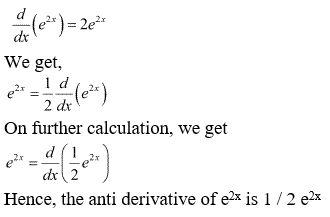
Example:
4. Methods of Integration(Integration by substitution)
- Books Name
- Mathmatics Book Based on NCERT
- Publication
- KRISHNA PUBLICATIONS
- Course
- CBSE Class 12
- Subject
- Mathmatics
Integration by Substitution:
Integration by substitution, also known as u-substitution, reverse chain rule or change of variables, is a method for evaluating integrals and antiderivatives. It is the counterpart to the chain rule for differentiation, and can loosely be thought of as using the chain rule "backwards".
The General Form of integration by substitution is:
Usually the method of integration by substitution is extremely useful when we make a substitution for a function whose derivative is also present in the integrand. Doing so, the function simplifies and then the basic formulas of integration can be used to integrate the function.
Example:
∫sin (x3).3x2.dx = ∫sin t . dt Let x3= t => 3x2dx =dt
= -cos t + c
Example :
Find the integration of

Solution:
Given : I =
Example :
Integrate 6x cos (x2 – 5) with respect to x .
Solution:
I = ∫6xcos(x2 – 5).dx
Let x2 – 5 = t …..(1)
2x.dx = dt
we have
I = 3∫cos(t).dt
= 3sin t + c …..(2)
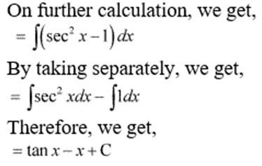
= 3sin (x2 – 5) + C
![]()
We know that tan x = sin x / cos x.
Therefore,
∫ tan x dx = ∫ (sin x / cos x) dx.
Now, let cos x = t, => sin x dx = – dt.
Therefore,
∫ tan x dx = – ∫ (dt / t) = – log |cos x| + C
Or, ∫ tan x dx = log |sec x| + C
![]()
We know that cot x = cos x / sin x. Therefore,
∫ cot x dx = ∫ (cos x / sin x) dx.
Now, let sin x = t, => cos x dx = – dt.
Therefore,
∫ cot x dx = ∫ (dt / t) = log |t| + C = log |sin x| + C
![]()
On multiplying both the numerator and denominator by (sec x + tan x), we have
∫ sec x dx = ∫ {sec x (sec x + tan x) dx} / (sec x + tan x)
Now, let (sec x + tan x) = t, => sec x (sec x + tan x) dx = dt.
Therefore, ∫ sec x dx = ∫ (dt / t) = log |t| + C = log |sec x + tan x| + C
![]()
On multiplying both the numerator and denominator by (cosec x + cot x), we have
∫ cosec x dx = ∫ {cosec x (cosec x + cot x) dx} / (cosec x + cot x)
Now, let (x + cot x) = t, => – cosec x (cosec x + cot x) dx = dt.
Therefore, ∫ cosec x dx = – ∫ (dt / t) = – log |t| + C = – log |cosec x + cot x| + C
= – log |(cosec2 x – cot2 x) / (cosec x – cot x)| + C
= log |cosec x – cot x| + C
Example :
Find the integral of (sin3 x) (cos2 x) dx
Solution: We have,
∫ (sin3 x) (cos2 x) dx = ∫ (sin2 x) (cos2 x) (sin x) dx
We know that sin2 x = (1 – cos2 x). we get
∫ (1 – cos2 x) (cos2 x) (sin x) dx
let cos x = t, =>t – sin x dx = dt.
Therefore,
∫ (1 – cos2 x) (cos2 x) (sin x) dx = – ∫ (1 – t2) t2 dt
= – ∫ (t2 – t4) dt
= – [(t3/3) – (t5/5)] + C
Hence, ∫ (sin3 x) (cos2 x) dx = – (1/3) cos3 x + (1/5) cos5 x + C
Integration using trigonometric identities:
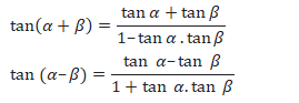
- sin(α+β)=sin(α). cos(β)+cos(α). sin(β)
- sin(α–β)=sinα. cosβ–cosα. sinβ
- cos(α+β)=cosα. cosβ–sinα. sinβ
- cos(α–β)=cosα. cosβ+sinα. sinβ
- sin 2θ = 2 sinθ cosθ
- cos 2θ = cos2θ – sin2 θ = 2 cos2θ – 1 = 1 – 2sin2 θ
- tan 2θ = (2tanθ)/(1 – tan2θ)
- sin (θ/2) = ±√[(1 – cosθ)/2]
- cos (θ/2) = ±√(1 + cosθ)/2
- tan (θ/2) = ±√[(1 – cosθ)(1 + cosθ)]
- Sin A. Sin B = [Cos (A – B) – Cos (A + B)]/2
- Sin A. Cos B = [Sin (A + B) – Sin (A – B)]/2
- Cos A. Cos B = [Cos (A + B) – Cos (A – B)]/2
- sin2 x + cos2 x = 1
1+tan2 x = sec2 x
cosec2 x = 1 + cot2 x - sin2 x =(1-cos2x)/2
- cos2 x =(1+cos2x)/2
tan2 x = sec2 x-1
cosec2 x - 1 = cot2 x - sin 3x = 3 sin x – 4 sin3 x,
- cos 3x = 4 cos3 x -3 cos x ,
Example :
Solve: ∫sin3x cos2x dx
Solution:
Given: ∫sin3x cos2x dx
∫sin3x cos2x dx = ∫sin2x sin x cos2x dx
We know that sin2x = 1-cos2x.
Therefore,
∫sin3x cos2x dx = ∫(1-cos2x)cos2x sinx dx
Now, let t = cos x, => dt = -sin x dx
Hence,
∫sin2x cos2x sin x dx = -∫(1-t2)t2 dt
= -∫(t2-t4) dt
∫sin2x cos2x sin x dx= -[(t3/3) -(t5/5)] + C
Now, let t = cos x, we get
∫sin2x cos2x sin x dx = -(⅓) cos3x + (⅕)cos5x + C
Therefore, ∫sin3x cos2x dx = -(⅓) cos3x + (⅕)cos5x + C.
Integrals of Some Particular Functions
Integral of function
we equate the coefficient of x of both the sides to determine the value of A and B, and hence the integral is reduced to one of the known forms.
Example: Find the Integral of the function ![]()
Solution:The given function can be converted into the standard form
5. Methods of Integration(Integration by Partial Fractions)
- Books Name
- Mathmatics Book Based on NCERT
- Publication
- KRISHNA PUBLICATIONS
- Course
- CBSE Class 12
- Subject
- Mathmatics
Integration by Partial Fractions
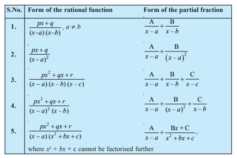
If f(x) and g(x) are polynomial functions such function. that g(x) ≠ 0 then f(x)/g(x) is called Rational Functions. If degree f(x) < degree g(x) then f(x)/g(x) is called a proper rational function then apply partial fraction method. If degree f(x) < degree g(x) then f(x)/g(x) is called an improper rational function. If f(x)/g(x) is an improper rational function then by dividing f(x) by g(x), we can express f(x)/g(x) as the sum of a polynomial and a proper rational function, then apply partial fraction method.
Partial Fractions
Any proper rational function p(x)/q(x) can be expressed as the sum of rational functions, each having the simplest factor q(x), each such fraction is known as a partial function and the process of obtaining them is called the decomposition or resolving of the given function into partial fractions.
Example : Evaluate ʃ (x – 1)/(x + 1)(x – 2) dx
Solution:
Let (x – 1)/(x + 1)(x – 2) = A/(x + 1) + B/(x – 2)
Then, (x – 1) = A(x – 2) + B(x + 1) ………………(i)
Putting x = -1 in (i), we get A = 2/3
Putting x = 2 in (i), we get B = 1/3
Therefore,
(x – 1)/(x + 1)(x – 2) = 2/3(x + 1) + 1/3(x – 2)
=> ʃ (x – 1)/(x + 1)(x – 2) = 2/3ʃdx/(x + 1) + 1/3ʃdx/(x – 2)
= 2/3log | x + 1 | + 1/3 log | x – 2 | + C
Example : Evaluate ʃdx/(x3 + x2 + x + 1)
Solution:
We have 1/(x3 + x2 + x + 1) = 1/x2(x + 1) + (x + 1) = 1/(x + 1)(x2 + 1)
Let 1/(x + 1)(x2 + 1) = A/(x + 1) + Bx + C/(x2 + 1) ……………………(i)
=> 1 ≡ A(x2 + 1) + (Bx + C) (x + 1)
Putting x = -1 on both sides of (i), we get A = 1/2.
Comparing coefficients of x2 on the both sides of (i), we get
A + B = 0 => B = -A = -1/2
Comparing coefficients of x on the both sides of (i), we get
B + C = 0 => C = -B = 1/2
Therefore, 1/(x + 1) (x2 + 1) = 1/2(x + 1) + (-1/2x + 1/2)/(x2 + 1)
Therefore, ʃ1/(x + 1) (x2 + 1) = ʃdx/(x + 1) (x2 + 1)
= 1/2ʃdx/(x + 1) – 1/2ʃx/(x2 + 1)dx + 1/2ʃdx/(x2 + 1)
= 1/2ʃdx/(x + 1) – 1/4ʃ2x/(x2 + 1)dx + 1/2ʃdx/(x2 + 1)
= 1/2 log | x + 1 | – 1/4 log | x2 + 1 | + 1/2 tan-1x + C
Example : Evaluate ʃx2/(x2 + 2)(x2 + 3)dx
Solution:
Let x2/(x2 + 2) (x2 + 3) = y/(y + 2)(y + 3) where x2 = y.
Let y/(y + 2) (y + 3) = A/(y + 2) + B/(y + 3)
=> y ≡ A(y + 3) + B/(y + 2) ………………(i)
Putting y = -2 on the both sides of (i), we get A = -2.
Putting y = -3 on the both sides of (i), we get B = 3.
Therefore, y/(y + 2) (y + 3) = -2/(y + 2) + 3/(y + 3)
=> x2/(x2 + 2) (x2 + 3) = -2/(x2 + 2) + 3/(x2 + 3)
=> ʃx2/(x2 + 2) (x2 + 3) = -2ʃdx/(x2 + 2) + 3ʃdx/(x2 + 3)
= -2/√2tan-1(x/√2) + 3/√3tan-1(x/√3) + C
= -√2tan-1(x/√2) + √3tan-1(x/√3) + C
Example : Evaluate ʃdx/x(x4 + 1)?
Solution:
We have
I = ʃdx/x(x4 + 1) = ʃx3/x4 (x4 + 1) dx [multiplying numerator and denominator by x3].
Putting x4 = t and 4x3dx = dt, we get
I = 1/4ʃdt/t(t + 1)
= 1/4∫{1/t – 1/(t + 1)}dt [by partial fraction]
= 1/4ʃ1/t dt – 1/4ʃ1/(t + 1)dt
= 1/4 log | t | – 1/4 log | t + 1 | + C
= 1/4 log | x4 | – 1/4 log | x4 + 1 | + C
= (1/4 * 4) log | x | – 1/4 log | x4 + 1 | + C
= log | x | – 1/4 log | x4 + 1 | + C
6. Methods of Integration(Integration by Parts)
- Books Name
- Mathmatics Book Based on NCERT
- Publication
- KRISHNA PUBLICATIONS
- Course
- CBSE Class 12
- Subject
- Mathmatics
Integration by Parts
∫f(x) g(x) dx = f(x)∫g(x)dx – ∫[f'(x)∫g(x)dx]dx
This is the basic formula which is used to integrate products of two functions by parts.
If we consider f as the first function and g as the second function, then this formula may be pronounced as:
“The integral of the product of two functions = (first function) × (integral of the second function) – Integral of [(differential coefficient of the first function) × (integral of the second function)]”.
ILATE Rule
Identify the function that comes first on the following list and select it as f(x).
ILATE stands for:
I: Inverse trigonometric functions : tan-1 x, sec-1 x, sin-1 x etc.
L: Logarithmic functions : ln x, log5(x), etc.
A: Algebraic functions. such as,x ,x2 etc..
T: Trigonometric functions, such as sin x, cos x, tan x etc.
E: Exponential functions.

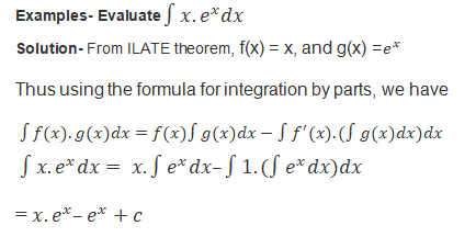
Example : Find ∫ x cos x dx
Solution: Let, The first function = f(x) = x and the second function = g(x) = cos x. Therefore, according to integration by parts, we have
∫ x cos x dx = x ∫ cos x dx – ∫ [(dx/dt) ∫ cos x dx] dx = x sin x – ∫ sin x dx
= x sin x + cos x + C.
Let’s try the other way round. Let, the first function = f(x) = cos x and the second function = g(x) = x. Therefore,
∫ x cos x dx = cos x ∫ x dx – ∫ {[d(cos x)/ dx] ∫ x } dx
= (cos x) (x2/2) + ∫ (sin x) (x2/2) dx
Example 2: Find ∫ log x dx
Solution: Do you know any function whose derivative is log x? Guessing it is difficult. Hence, let’s take the first function f(x) = log x. So, the second function g(x) = 1. And, we know that ∫ 1 dx = x. Therefore, ∫ g(x) dx = x. Therefore, we have,
Example: ![]()
Solution:

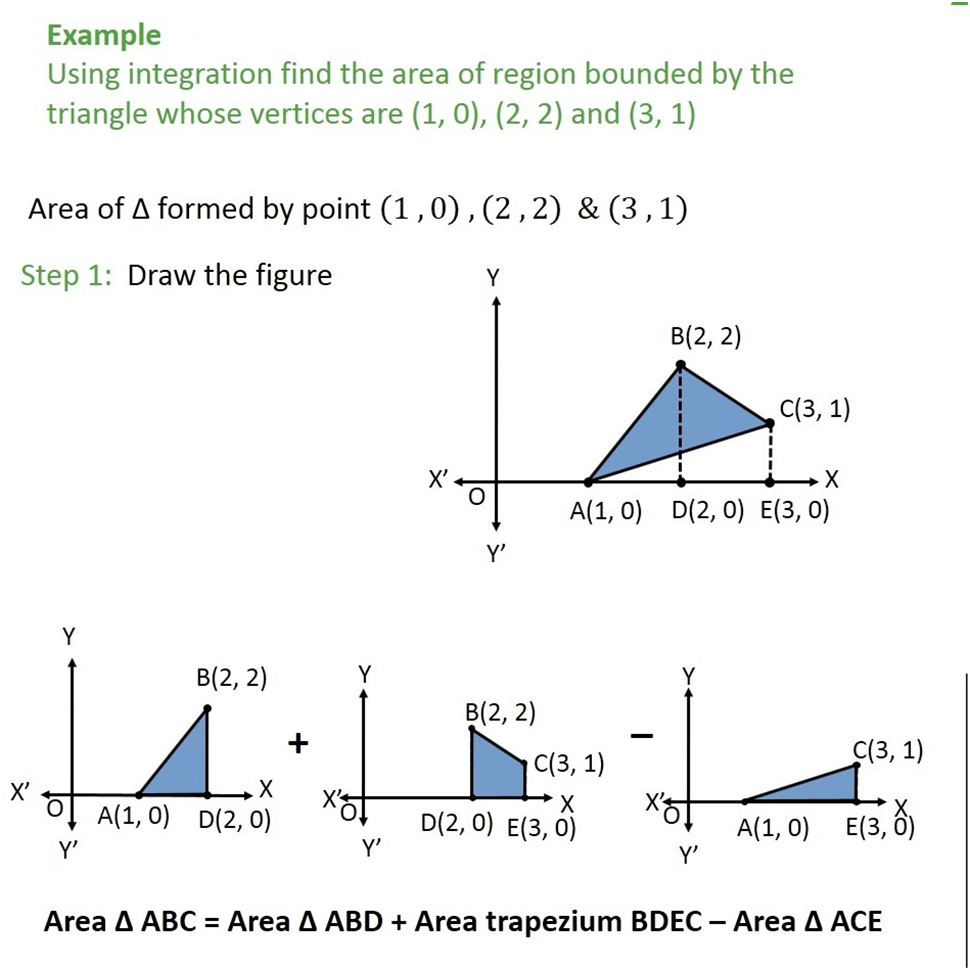
2. The area of the region bounded by a curve and a line
- Books Name
- Mathmatics Book Based on NCERT
- Publication
- KRISHNA PUBLICATIONS
- Course
- CBSE Class 12
- Subject
- Mathmatics
To find the area of the region bounded by a curve and a line
Let’s have a look at the example to understand how to find the area of the region bounded by a curve and a line.
Example 2:
Find the area of the region bounded between the line x = 2 and the parabola y2 = 8x.
Solution:
Given equation of parabola is y2 = 8x.
Equation of line is x = 2.
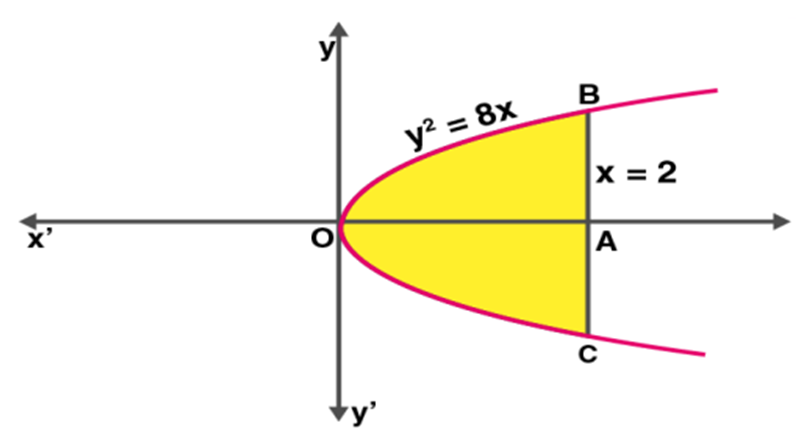
Here, y2 = 8x as a right handed parabola having its vertex at the origin and x = 2 is the line which is parallel to y-axis at x = 2 units distance
Similarly,
y2 = 8x has only even power of y and is symmetrical about x-axis.
So, the required area = Area of OAC + Area of OAB
= 2 (Area of OAB)
= 2 ∫02 y dx
Substituting the value of y, i.e. y2 = 8x and y = √(8x) = 2 √2 √x, we get;
= 2 ∫02 (2 √2 √x) dx
= 4√2 ∫02 (√x) dx
= 4√2 [x3/2/ (3/2)]02
By applying the limits,
= 4√2 {[23/2/ (3/2)] – 0}
= (8√2/3) × 2√2
= (16 × √2 × √2)
= 32/3
Go through the example given below to learn how to find the area between two curves.
Example 3:
Determine the area which lies above the x-axis and included between the circle and parabola, where the circle equation is given as x2+y2 = 8x, and parabola equation is y2 = 4x.
Solution:
The circle equation x2+y2 = 8x can be written as (x-4)2+y2=16. Hence, the centre of the circle is (4, 0), and the radius is 4 units. The intersection of the circle with the parabola y2 = 4x is as follows:
Now, substitute y2 = 4x in the given circle equation,
x2+4x = 8x
x2– 4x = 0
On solving the above equation, we get
x=0 and x=4
Therefore, the point of intersection of the circle and the parabola above the x-axis is obtained as O(0,0) and P(4,4).
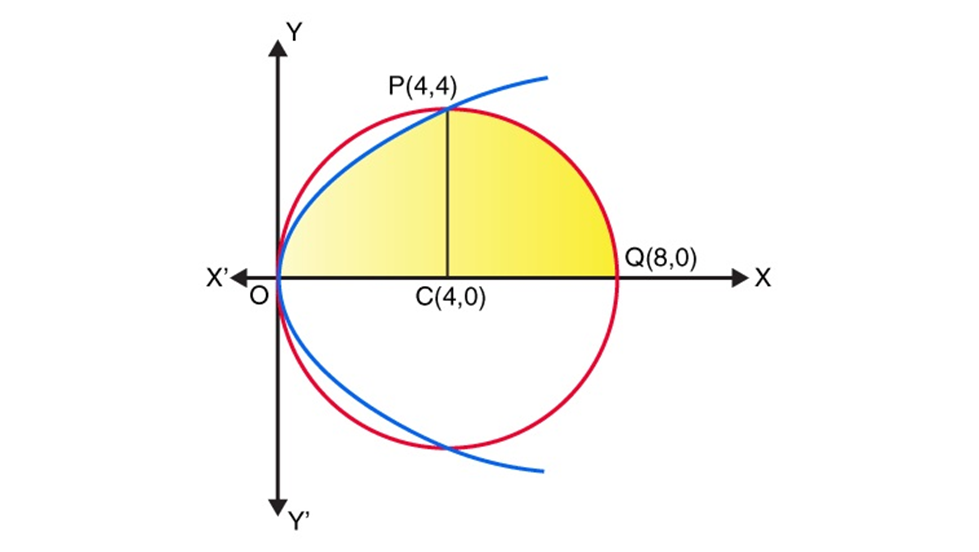
Hence, from the above figure, the area of the region OPQCO included between these two curves above the x-axis is written as
= Area of OCPO + Area of PCQP
= 0∫4 y dx + 4∫8 y dx
= 2 0∫4 √x dx + 4∫8 √[42– (x-4)2]dx
Now take x-4 = t, then the above equation is written in the form
= 2 0∫4 √x dx + 0∫4 √[42– t2]dx …. (1)
Now, integrate the functions.
2 0∫4 √x dx = (2)(⅔) (x3/2)04
2 0∫4 √x dx = 32/3 …..(2)
0∫4 √[42– t2]dx = [(t/2)(√[42-t2] + (½)(42)(sin-1(t/4)]04
0∫4 √[42– t2]dx = 4π …..(3)
Now, substitute (2) and (3) in (1), we get
= (32/3) + 4π
= (4/3) (8+3π)
Therefore, the area of the region that lies above the x-axis, and included between the circle and parabola is (4/3) (8+3π).
3. Area between Two Curves
- Books Name
- Mathmatics Book Based on NCERT
- Publication
- KRISHNA PUBLICATIONS
- Course
- CBSE Class 12
- Subject
- Mathmatics
Area Between Two Curves
Type-1:
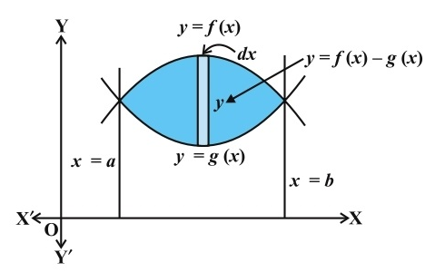
Area between two curves = ∫ab [f(x) – g(x)] dx
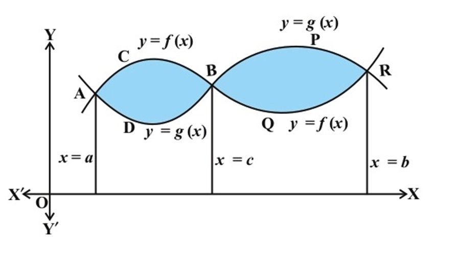
Type-2:
Example:
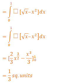
Find the area of the region bounded by the parabolas y = x2 and x = y2.
Solution:
When the graph of both the parabolas is sketched we see that the points of intersection of the curves are (0, 0) and (1, 1) as shown in the figure below.
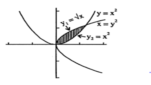
So, we need to find the area enclosed between these points which would give us the area between two curves. Also, in the given region as we can see,
y = x2 = g(x)
and
x = y2
or, y = √x = f(x).
As we can see in the given region,
The area enclosed will be given as,
Example :
Find the area bounded by curves (x – 1)2 + y2 = 1 and x2 + y2 = 1.
Solution:
Given equations of curves:
x2 + y2 = 1 ….(i)
(x – 1)2 + y2 = 1 ….(ii)
From (i),
y2 = 1 – x2
By substituting it in equation (2), we get;
(x – 1)2 + 1 – x2 = 1
On further simplification
(x – 1)2 – x2 = 0
Using the identity a2 – b2 = (a – b)(a + b),
(x – 1 – x) (x – 1 + x) = 0
-1(2x – 1) = 0
– 2x + 1 = 0
2x = 1
x = 1/2
Using this in equation (1) we get;
y = ± √3/2
Thus, both the equations intersect at point A (1/2, √3/2) and B (1/2, -√3/2).
Also, (0, 0) is the centre of first circle and radius 1
Similarly, (1, 0) is the centre of second circle and radius is 1.
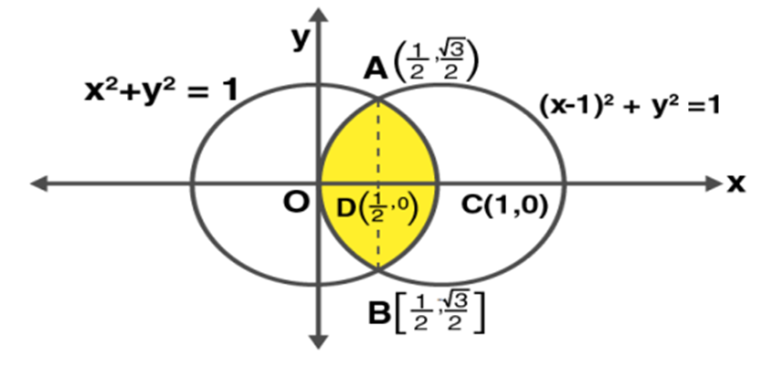
Here, both the circles are symmetrical about x-axis and the required area is shaded here.
So, the required area = area OACB
= 2 (area OAC)
= 2 [area of OAD + area DCA]
2. Order and Degree of a differential equation
- Books Name
- Mathmatics Book Based on NCERT
- Publication
- KRISHNA PUBLICATIONS
- Course
- CBSE Class 12
- Subject
- Mathmatics
Order and Degree of a differential equation
What is ODE and PDE?
Ordinary differential equations or (ODE) are equations where the derivatives are taken with respect to only one variable. That is, there is only one independent variable. Partial differential equations or (PDE) are equations that depend on partial derivatives of several variables.
Order of differential equation
The highest order of the derivative present in the dependent variable with respect to the independent variable in the given differential equation is called order of DE.
Degree of differential equation
Degree of the differential equation is the exponent of the highest derivative of the differential equation
Example:
Example:
![]()
order=2, degree=not defined because it is not a polynomial function.
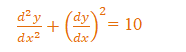
Example:
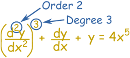
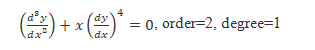
order=2 ,degree=3
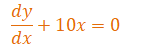
Example :
![]()
Here, the exponent of the highest order derivative is one and the given differential equation is a polynomial equation in derivatives. Hence, the degree of this equation is 1.
Example :
The order of this equation is 3 and the degree is 2 as the highest derivative is of order 3 and the exponent raised to the highest derivative is 2.
Order and degree (if defined) of a differential equation are always positive integers.
3. General and Particular Solutions of a Differential Equation
- Books Name
- Mathmatics Book Based on NCERT
- Publication
- KRISHNA PUBLICATIONS
- Course
- CBSE Class 12
- Subject
- Mathmatics
General and Particular Solution of a Differential Equation
General(or primitive) solution:
The solution which contains arbitrary constants is called the general(or primitive) solution of the differential equation.
The general solution of the differential equation is of the form y = f(x) or y = ax + b and it has a, b as its arbitrary constants.
Example:
The function y = a cos x + b sin x, where, a, b Î R is a solution
of the differential equation
![]()
Particular solution:
The solution free from arbitrary constants obtained from the general solution by giving particular values to the arbitrary constants is called a particular solution of the differential equation.
Example: y = e– 3x is a particular solution of the differential equation
![]()
Example : The number of arbitrary constants in the general solution of a differential equation
of fourth order are:
- 0
- 2
- 3
- 4
Ans: D
Example: The number of arbitrary constants in the particular solution of a differential equation
of third order are:
- 3
- 2
- 1
- 0
Ans: D
4. Formation of a Differential Equation whose General Solution is given
- Books Name
- Mathmatics Book Based on NCERT
- Publication
- KRISHNA PUBLICATIONS
- Course
- CBSE Class 12
- Subject
- Mathmatics
Formation of a Differential Equation whose General Solution is given
The order of a differential equation representing a family of curves is the same as the number of arbitrary constants present in the equation corresponding to the family of curves.
Procedure to form a differential equation that will represent a given
family of curves:
(a) If the given family F1 of curves depends on only one parameter then it is
represented by an equation of the form
F1 (x, y, a) = 0 ... (1)
For example, the family of parabolas y2 = ax can be represented by an equation of the form
f (x, y, a) : y2 = ax.
Differentiating equation (1) with respect to x, we get an equation involving y', y, x, and a,
i.e.,
g (x, y, y', a) = 0 ................ (2)
The required differential equation is then obtained by eliminating a from equations (1) and (2) as
F(x, y, y' ) = 0 ..................... (3)
(b) If the given family F2 of curves depends on the parameters a, b (say) then it is represented by an equation of the from
F2 (x, y, a, b) = 0 …………………….(4)
Differentiating equation (4) with respect to x, we get an equation involving ![]() , x, y, a, b,
, x, y, a, b,
i.e.,
g (x, y, y'', a, b) = 0 ………………………(7)
But it is not possible to eliminate two parameters a and b from the two equations and so, we need a third equation. This equation is obtained by differentiating equation (5), with respect to x, to obtain a relation of the form
h (x, y, y',
The required differential equation is then obtained by eliminating a and b from equations (4), (5) and (6) as
F (x, y, y',
Note: The order of a differential equation representing a family of curves is same as the number of arbitrary constants present in the equation corresponding to the family of curves.
Example : Form the differential equation representing the family of curves y = mx,
where, m is arbitrary constant.
Solution: We have
y = mx ... …………………(1)
Differentiating both sides of equation (1) with respect to x, we get
y’ = m
Substituting the value of m in equation (1) we get
y= y’ x
- xy’-y=0
which is free from the parameter m and hence this is the required differential equation.
Example : Form the differential equation representing the family of curves
y = a sin (x + b), where a, b are arbitrary constants.
Solution :We have
y = a sin (x + b) ... ……………(1)
Differentiating both sides of equation (1) with respect to x, successively we get
y’ =a cos(x+b)…………………..(2)
- y’’ = -a sin(x+b)………………….(3)
Eliminating a and b from equations (1), (2) and (3), we get
y’’ +y =0 ………………………(4)
which is free from the arbitrary constants a and b and hence this the required differential equation.
7. Integrals of some more types
- Books Name
- Mathmatics Book Based on NCERT
- Publication
- KRISHNA PUBLICATIONS
- Course
- CBSE Class 12
- Subject
- Mathmatics
Integrals of some more types
- ∫ √(x2 - a2) dx
- ∫ √(a2 - x2) dx
- ∫ √(x2 + a2) dx
Proof:
[1] ∫ √(x2 - a2) dx
Let I = ∫ √(x2 - a2) dx
⇒I = ∫ 1. √(x2 - a2) dx
⇒I = ∫ √(x2 - a2) . 1dx
Let f(x) = √(x2 - a2) and g(x) = 1
∫ f(x) g(x) dx = f(x) ∫ g(x) dx - ∫ [ f '(x) ∫ g(x) dx] dx
Thus ∫ √(x2 - a2) . 1dx = √(x2 - a2) . ∫ 1 dx - ∫ [d/dx(√(x2 - a2)) ∫1dx] dx
⇒ I = √(x2 - a2) . x - ∫ 1/(2(√(x2 - a2))) . 2x .x dx
⇒ I = x√(x2 - a2) - ∫ x2/√(x2 - a2) dx
⇒ I = x√(x2 - a2) - ∫ (x2 - a2 + a2)/√(x2 - a2) dx
⇒ I = x√(x2 - a2) - ∫ (x2 - a2)/√(x2 - a2) dx - ∫ a2/√(x2 - a2) dx
⇒ I = x√(x2 - a2) - ∫ √(x2 - a2) dx - ∫ a2/√(x2 - a2) dx
⇒ I = x √(x2 - a2) - I - ∫ a2/√(x2 - a2) dx
⇒ 2I = x √(x2 - a2) - a2 ∫ 1/√(x2 - a2) dx
⇒ 2I = x √(x2 - a2) - a2 log|x + √(x2 - a2)| + C
⇒ I = x/2 . √(x2 - a2) - a2/2 . log|x + √(x2 - a2)| + C
Note: The integral of √(x2 - a2) can also be evaluated by substituting x = a sec θ.
[2] ∫ √(x2 + a2) dx
Let I = ∫ √(x2 + a2) . 1dx
Let f(x) = √(x2 + a2) and g(x) =1
∫ f(x) g(x) dx = f(x) ∫ g(x) dx - ∫ [ f '(x) ∫ g(x) dx] dx
I = √(x2 + a2) ∫ 1 dx - ∫ [d/dx (√(x2 + a2)) ∫ 1dx] dx
⇒ I = √(x2 + a2) . x - ∫ 1/(2√(x2 + a2)). 2x . x dx
⇒ I = x √(x2 + a2) - ∫ x2/√(x2 + a2) dx
⇒ I = x √(x2 + a2) - ∫ (x2 + a2 - a2)/√(x2 + a2) dx
⇒ I = x√(x2 + a2) - ∫ (x2 - a2)/√(x2 + a2) dx + ∫ a2/√(x2 + a2) dx
⇒ I = x√(x2 + a2) - ∫ √(x2 + a2) dx + ∫ a2/√(x2 + a2) dx
⇒ I = x √(x2 + a2) - I + ∫ a2/√(x2 + a2) dx
⇒ 2I = x √(x2 + a2) + ∫ a2 /√(x2 + a2) dx
⇒ 2I = x √(x2 + a2) + a2 ∫ 1 /√(x2 + a2) dx
⇒ 2I = x √(x2 - a2) + a2 log|x + √(x2 + a2)| + C
⇒ I = x/2 . √(x2 + a2) + a2/2 . log|x + √(x2 + a2)| + C
Note: The integral of √(x2 + a2) can also be evaluated by substituting x = a tan θ.
[3] Let I= ∫ √(a2 - x2) dx
= ∫ √(a2 - x2) . 1 dx
= ∫ √(a2 - x2) . 1dx
Let f(x) = √(a2 - x2) and g(x) = 1
∫ f(x) g(x) dx = f(x) ∫ g(x) dx - ∫ [ f '(x) ∫ g(x) dx] dx
= √(a2 - x2) ∫ 1dx - ∫ [d/dx (√(a2 - x2)) ∫ 1dx] dx
⇒ I = √(a2 - x2) . x - ∫ 1/2(√(a2 - x2)) . (-2x) . x dx
⇒ I = x√(a2 - x2) - ∫ -x2/√(a2 - x2) dx
⇒ I = x√(a2 - x2) - ∫ ((a2-x2)-a2)/√(a2 - x2) dx
⇒ I = x√(a2 - x2) - ∫ (a2-x2)/√(a2 - x2) dx + ∫ a2/√(a2 - x2) dx
⇒ I = x√(a2 - x2) - ∫ √(a2 - x2) dx + ∫ a2/√(a2 - x2) dx
⇒ I = x√(a2 - x2) - I + ∫ a2/√(a2 - x2) dx
⇒ 2I = x√(a2 - x2) + a2 ∫ 1/√(a2 - x2) dx
⇒ 2I = x√(a2 - x2) + a2 sin-1 (x/a) + C
⇒ I = x/2 √(a2 - x2)+ a2/2 sin-1 (x/a) + C
Note: The integral of √(a2 - x2) can also be evaluated by substituting x = a sin θ.
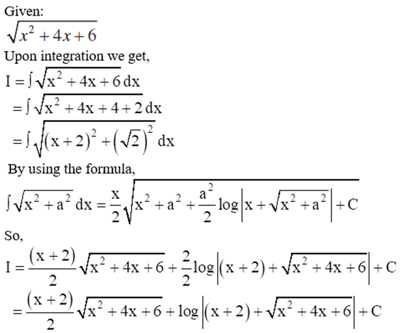
8. Concept of Definite Integral and Definite Integral as the limit of a sum
- Books Name
- Mathmatics Book Based on NCERT
- Publication
- KRISHNA PUBLICATIONS
- Course
- CBSE Class 12
- Subject
- Mathmatics
Definite Integral
A definite integral is denoted by ∫ab f(x) dx, where a is called the lower limit of the integral and b is called the upper limit of the integral.
Definite Integral as the limit of a sum:
The integral of f(x) is the area of the region bounded by the curve y = f(x). This area is represented by the region ABCD as shown in the above figure. This entire region lying between [a, b] is divided into n equal subintervals given by [x0, x1], [x1, x2], …… [xr-1, xr], [xn-1, xn].
Let us consider the width of each subinterval as h such that h → 0, x0 = a, x1 = a + h, x2 = a + 2h,…..,xr = a + rh, xn = b = a + nh
and n = (b – a)/h
Also, n→∞ in the above representation.
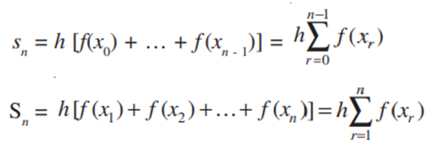
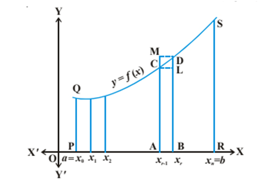
Since, n→∞, the rectangular strips are very narrow, it can be assumed that the limiting values of sn and Sn are equal and the common limiting value gives us the area under the curve, i.e.,
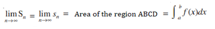
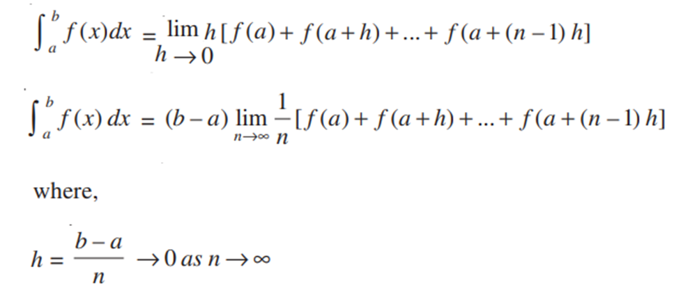
Question : Find ∫ab x dx as the limit of a sum.
Answer : From equation (6) above, we know that
∫ab f(x) dx = (b – a) limn → ∞ (1/n) [f(a) + f(a + h) + …. + f(a + {n – 1}h)]
Where, h = (b – a)/n
In this example, we have
a = a, b = b, f(x) = x and h = (b – a)/n.
Also, f(a) = a
f(a + h) = a + h
f(a + 2h) = a + 2h
f(a + 3h) = a + 3h ……
f(a + (n – 1)h) = a + (n – 1)h
Therefore,
∫ab x dx = (b – a) limn → ∞ (1/n) [f(a) + f(a + h) + f(a + 2h) + …. + f(a + {n – 1}h)]
= (b – a) limn → ∞ (1/n) [a + (a + h) + (a + 2h) + …. + (a + (n – 1)h)]
= (b – a) limn → ∞ (1/n) {[a + a + a + … + a(n-times)] + h + 2h + …. + (n – 1)h}
= (b – a) limn → ∞ (1/n) [na + h(1 + 2 + ….. + (n – 1)]
Now, we know that, 1 + 2 + 3 + … + n = n(n + 1)/2. Hence,
1 + 2 + 3 + … + (n – 1) = (n – 1)(n – 1 + 1)/2 = n(n – 1)/2
Therefore,
∫ab x dx = (b – a) limn → ∞ (1/n) [na + hn(n – 1)/2]
= (b – a) limn → ∞ [na/n + hn(n – 1)/2n]
= (b – a) limn → ∞ [a + (n – 1)h/2]
Replacing h by (b – a)/n, we get
∫ab x dx = (b – a) limn → ∞ [a + (n – 1) (b – a) / 2n]
= (b – a) limn → ∞ [a + (n/n – 1/n) {(b – a)/2}]
= (b – a) limn → ∞ [a + (1 – 1/n){(b – a)/2}]
= (b – a) [a + (1 – 1/∞) {(b – a)/2}]
= (b – a) [a + (1 – 0){(b – a)/2}]
= (b – a) [a + (b – a)/2]
= (b – a) (2a + b – a)/2
= (b – a) (b + a)/2
= (b2 – a2)/2
Hence, the definite integral ∫ab x dx as the limit of sum is [(b2 – a2)/2].
Example: Find ∫02 (x2 + 1) dx as the limit of a sum.
Solution: From above, we know that
∫ab f(x) dx = (b – a) limn → ∞ (1/n) [f(a) + f(a + h) + …. + f(a + {n – 1}h)]
Where, h = (b – a)/n
we have a = 0, b = 2, f(x) = (x2 + 1) and h = (2 – 0)/n = 2/n. Therefore,
∫02 (x2 + 1) dx = 2 limn → ∞ (1/n) [f(0) + f(2/n) + f(4/n) + …. + f(2{n – 1}/n)]
= 2 limn → ∞ (1/n) [1 + {(22/n2) + 1} + {(42/n2) + 1} + …. + {(2n – 2)2/n2 + 1}]
= 2 limn → ∞ (1/n) [1 + 1 + 1 + … + 1(n-times)] + 1/n2) [22 + 42 + … (2n – 2)2]
= 2 limn → ∞ (1/n) [n + 22/n2 (12 + 22 + … (n – 1)2]
= 2 limn → ∞ (1/n) [n + 4/n2 {(n – 1) n (2n – 1) / 6}]
= 2 limn → ∞ (1/n) [n + 2/3 {(n – 1) (2n – 1) / n}]
= 2 limn → ∞ (1/n) [n + 2/3 (1 – 1/n) (2 – 1/n)]
As n → ∞, 1/n → 0. Therefore, we have
∫02 (x2 + 1) dx = 2 [1 + 4/3] = 14/3.
9. Fundamental Theorem of Calculus
- Books Name
- Mathmatics Book Based on NCERT
- Publication
- KRISHNA PUBLICATIONS
- Course
- CBSE Class 12
- Subject
- Mathmatics
Fundamental Theorem of Calculus
Fundamental theorem of calculus contains two important theorems namely:

First fundamental theorem of integral calculus
Let f be a continuous function on the closed interval [a, b] and let A (x) be the area function. Then A′(x) = f (x), for all x ∈ [a, b].
Second fundamental theorem of integral calculus
Let f be a continuous function defined on the closed interval [a, b] and F be an antiderivative of f.
Then ∫ab f(x) dx= [F(x)]ab = F(b) – F(a)
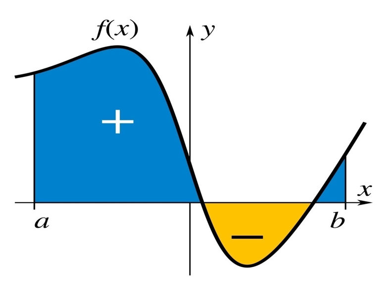
10. Evaluation of Definite Integrals by Substitution and more methods
- Books Name
- Mathmatics Book Based on NCERT
- Publication
- KRISHNA PUBLICATIONS
- Course
- CBSE Class 12
- Subject
- Mathmatics
Evaluation of Definite Integrals by Substitution and more methods:
To evaluate ![]() by substitution, the steps could be as follows:
by substitution, the steps could be as follows:
1. Consider the integral without limits and substitute, y = f (x) or x = g(y) to reduce
the given integral to a known form.
2. Integrate the new integrand with respect to the new variable without mentioning
the constant of integration.
3. Re-substitute for the new variable and write the answer in terms of the original
variable.
4. Find the values of answers obtained in (3) at the given limits of integral and find
the difference of the values at the upper and lower limits. Although we will not formally prove this theorem, we justify it with some calculations here. From the substitution rule for indefinite integrals, if F(x) is an anti-derivative of f(x) we have
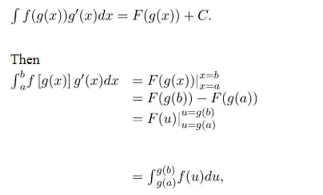
and we have the desired result.Using substitution to evaluate a definite integral requires a change to the limits of integration. If we change variables in the integrand, the limits of integration change as well.
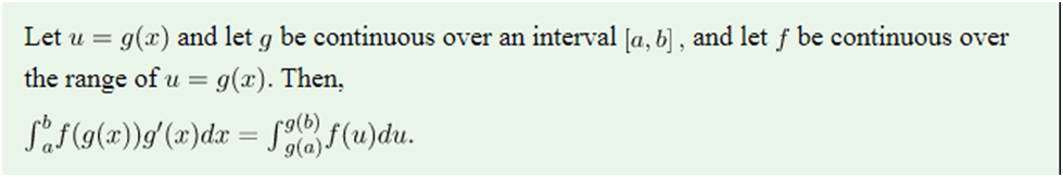

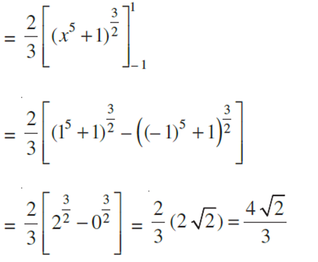
Alternatively, first we transform the integral and then evaluate the transformed integral with new limits.
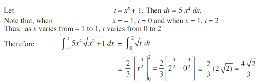
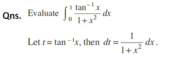
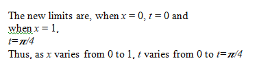
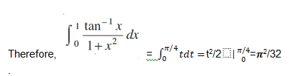
11. Some Properties of Definite Integrals and evaluation of definite integrals
- Books Name
- Mathmatics Book Based on NCERT
- Publication
- KRISHNA PUBLICATIONS
- Course
- CBSE Class 12
- Subject
- Mathmatics
Some Properties of Definite Integrals and evaluation of definite integrals
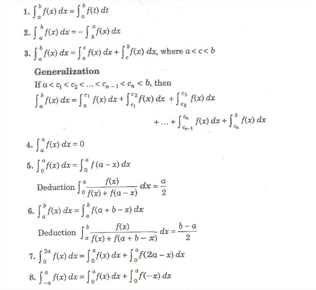
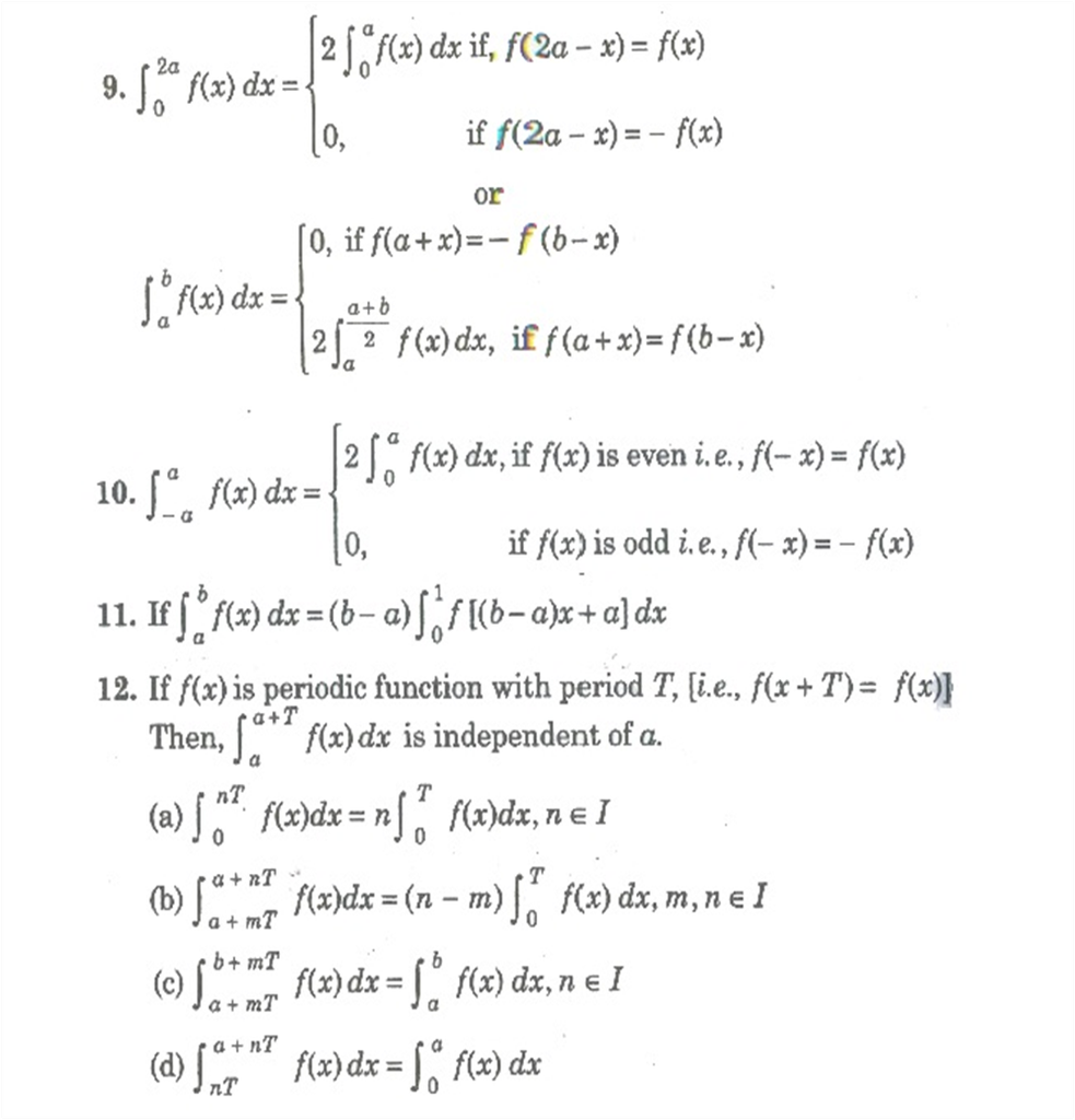
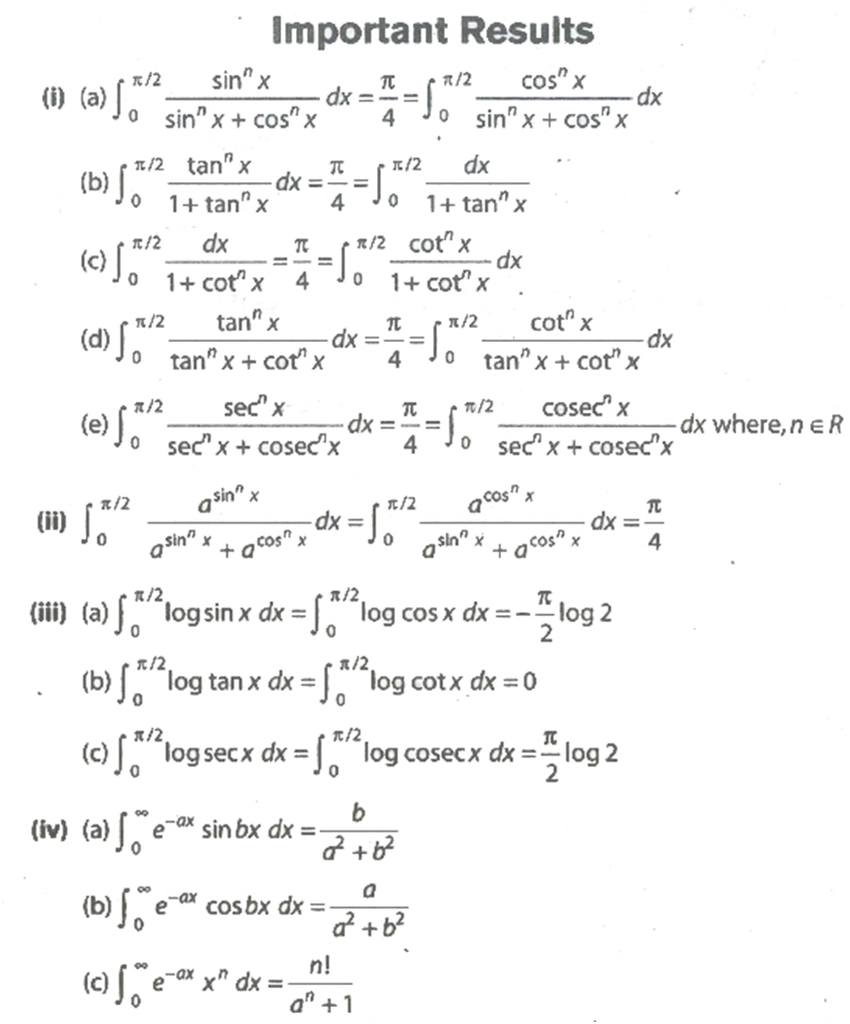
Example :
Prove that 0∫π/2 (2log sinx – log sin 2x)dx = – (π/2) log 2
Solution:
To prove: 0∫π/2 (2log sinx – log sin 2x)dx = – (π/2) log 2
Proof:
Let I = 0∫π/2 (2log sinx – log sin 2x)dx ………………………….…(1)
By using the property of definite integral
0∫a f(x) dx = 0∫a f(a-x) dx
Now, apply the property in (1), we get
-
- I = 0∫π/2 2log sin[(π/2)-x] – log sin 2[(π/2)-x])dx
The above expression can be written as
-
- I = 0∫π/2 [2log cosx- log sin(π-2x)]dx (Since, sin (90-θ = cos θ)
- I = 0∫π/2 [2log cosx- log sin2x]dx ……………………………………………………..(2)
Now, add the equation (1) and (2), we get
-
- I+ I = 0∫π/2 [(2log sinx – log sin 2x) +(2log cosx- log sin2x)]dx
- 2I = 0∫π/2 [2log sinx -2log 2sinx + 2log cos x]dx
- 2I = 2 0∫π/2 [log sinx -log 2sinx + log cos x]dx
-
- = 0∫π/2 [log sinx + log cos x- log 2sinx]dx
-
- I = 0∫π/2log[(sinx. cos x)/sin2x]dx
We know that sin2x= 2 sinx cos x)
-
- I = 0∫π/2log[(sinx. cos x)/(2 sinx cos x)]dx
- I = 0∫π/2 log(1/2)dx
- I = 0∫π/2 (log1-log 2)dx [Since, log (a/b) = log a- log b]
- I = 0∫π/2 -log 2 dx (value of log 1 = 0)
Now, take the constant – log 2 outside the integral,
-
- I = -log 2 0∫π/2dx
Now, integrate the function
-
- I = -log 2 [x]0π/2
Now, substitute the limits
-
- I = -log 2 [(π/2)-0]
- I = – log 2 (π/2)
- I = – (π/2) log 2 = R.H.S
Therefore, L.H. S = R.H.S
Hence. 0∫π/2 (2log sinx – log sin 2x)dx = – (π/2) log 2 is proved.
Example: solve ![]()
Solution:
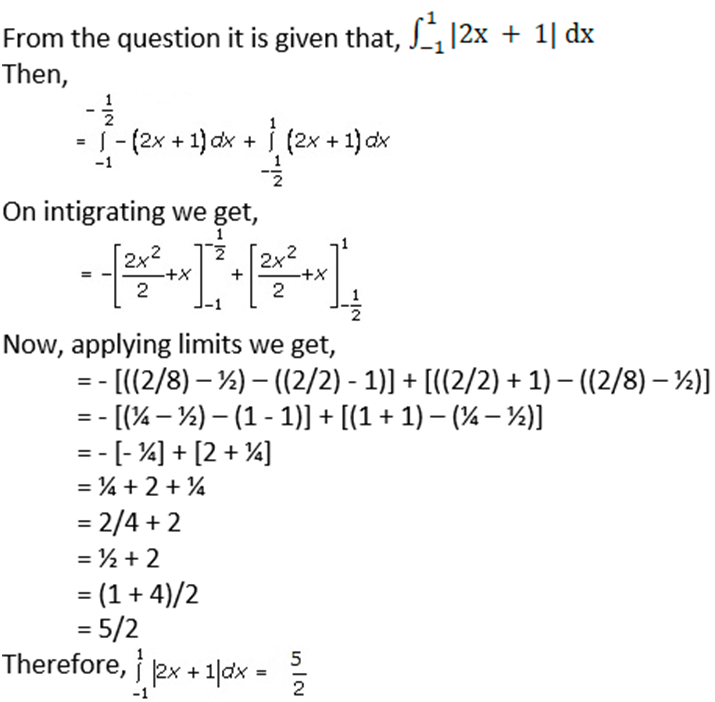
Question. 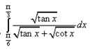
Solution:
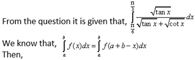
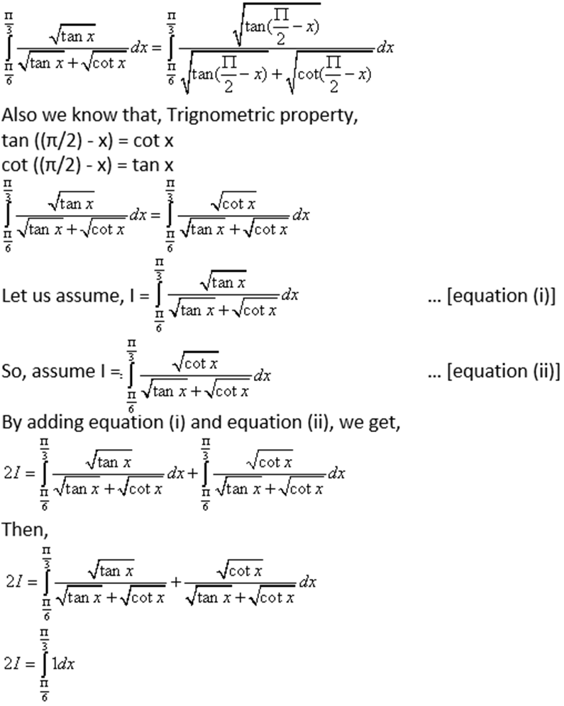
Now applying limits, we get,
2I = π/3 – π/6
2I = (2π – π)/6
2I = π/6
I = π/12
Question. 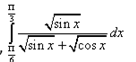
Solution:
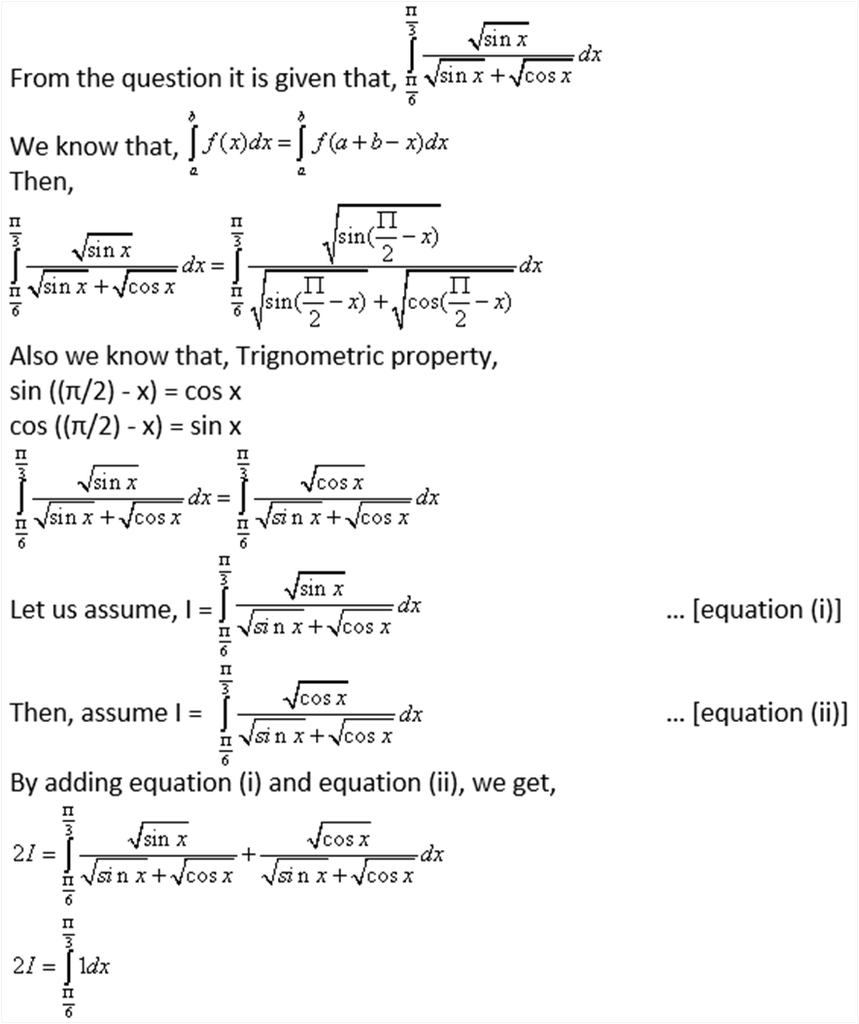
Now applying limits, we get,
2I = π/3 – π/6
2I = (2π – π)/6
2I = π/6
I = π/12
Question. 
Solution:
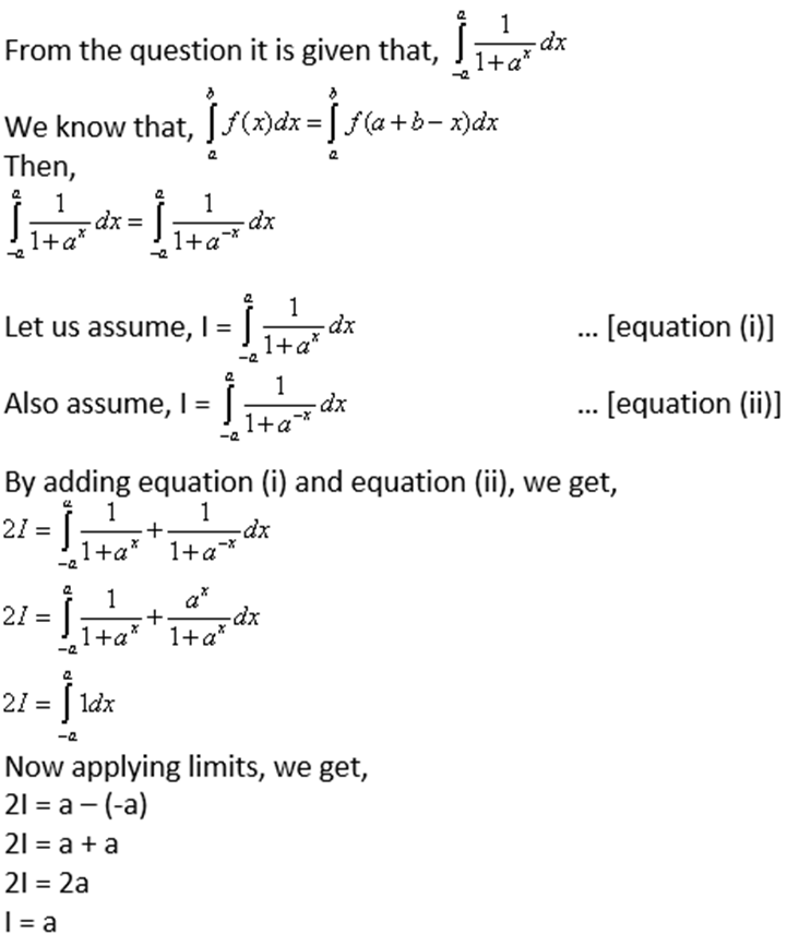
Question. 
Solution:
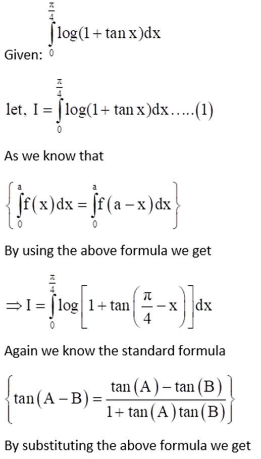
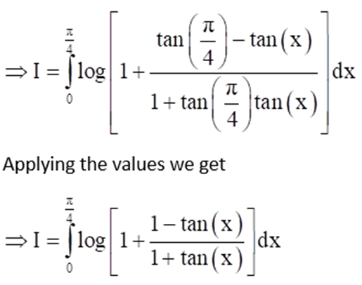
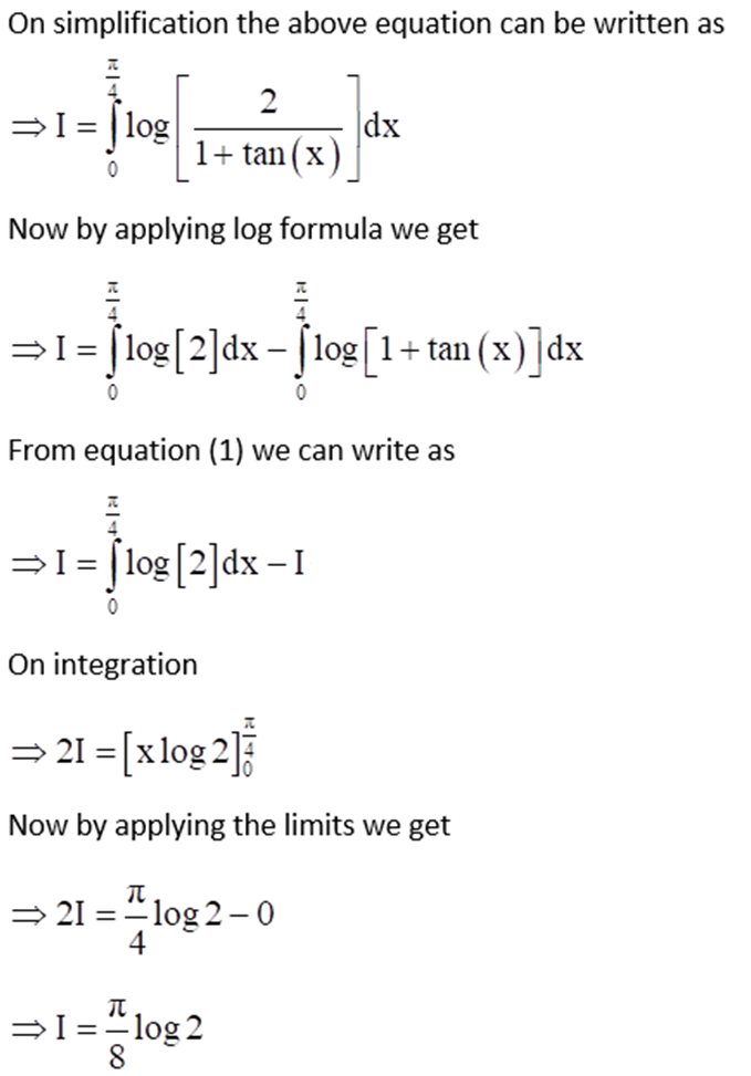
5. Methods of Solving First Order, First Degree Differential Equations and Differential equations with variables separable
- Books Name
- Mathmatics Book Based on NCERT
- Publication
- KRISHNA PUBLICATIONS
- Course
- CBSE Class 12
- Subject
- Mathmatics
Methods of Solving First Order, First Degree Differential Equations
There are three methods to solve the first-order, first-degree differential equations. They are:
- Differential equations with variables separable
- Homogeneous differential equations
- Linear differential equations
Differential equations with variables separable:
A first order-first degree differential equation is of the form
If F (x, y) can be expressed as a product g (x) h(y), where, g(x) is a function of x and h(y) is a function of y, then the differential equation (1) is said to be of variable separable type. The differential equation (1) then has the form
![]()
If h (y) ¹0, separating the variables, (2) can be rewritten as
![]()
Integrating both sides of (3), we get
Thus, (4) provides the solutions of given differential equation in the form
H(y) = G(x) + C
Example: Find the general solution of the differential equation ![]()
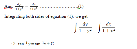
which is the general solution of equation (1).
6. Solutions of homogeneous differential equations of first order and first degree
- Books Name
- Mathmatics Book Based on NCERT
- Publication
- KRISHNA PUBLICATIONS
- Course
- CBSE Class 12
- Subject
- Mathmatics
Homogeneous differential equations
A function F(x, y) is said to be homogeneous function of degree n if
F(λx, λy) = λnF(x, y) for any nonzero constant λ .
A differential equation of the form ![]() is said to be homogenous if F(x, y) is a homogenous function of degree zero. We make the substitution y = v . x
is said to be homogenous if F(x, y) is a homogenous function of degree zero. We make the substitution y = v . x
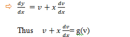
Separating the variables in equation , we get
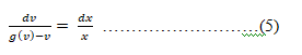
Integrating both sides of equation (5), we get
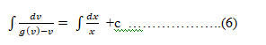
Equation (6) gives general solution (primitive) of the differential equation (1) when
we replace v by y/x.
Example: Solve dy/dx = (x-y)/(x+y)
Solution: Given, dy/dx = (x-y)/(x+y)
It is homogeneous degree 0.
![]()
Then,
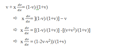
Now we can use the separation of variables method;
(1+v)/(1-2v-v2) dv = (1/x) dx
Integrating both the sides;
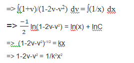
Again, putting v = y/x;
1-2(y/x)-(y/x)2 = 1/k2x2
Eliminating x2 term from denominator on both the sides, we get;
x2-2xy-y2 = 1/k2
or
y2+2xy-x2 = -1/k2
Now, put -/k2 = c
Adding 2x2 on both the sides;
y2+2xy+x2 = c+2x2
Now factoring the above equation, we get;
(y+x)2 = 2x2+c
y+x=√(2x2)+c
Or y = ±√(2x2+c) − x
This is the solution for the given equation.
Example: Find the equation of the curve passing through the point (1,-2) when the tangent at any point is given by ![]()
Solution: The equation of tangent represents the slope of the curve i.e.
This equation is homogeneous in nature.
On cross-multiplication, we get- ![]()
Solving the equation, we get
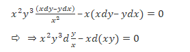
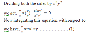
Now substituting the value of the given point in the above equation, we have
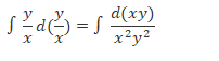
Put this value of the constant C in equation (1) we get
This is the required solution.
7. Solutions of linear differential equation of first order and first degree
- Books Name
- Mathmatics Book Based on NCERT
- Publication
- KRISHNA PUBLICATIONS
- Course
- CBSE Class 12
- Subject
- Mathmatics
Solutions of linear differential equation of first order and first degree
[1] A differential equation of the from
![]()
Where p,q are constants or functions of x, is known as a first order linear differential equation.
Integrating Factor(I.F.) of the given differential equation = g(x) ![]()
Write the solution of the given differential equation as
The general solution of the given differential equation as
![]()
[2] A differential equation of the from
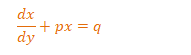
Where p,q are constants or functions of y, is known as a first order linear differential equation.
![]()
Write the solution of the given differential equation as
The general solution of the given differential equation as
![]()
Example :
Solve the following differential equation: