3. Graphical method of solving linear programming problems

Graphical method of solving linear programming problems

This section comprises the definition of the feasible region, feasible solution and infeasible solution, optimal solution, bounded and unbounded region of feasible solution.

The graphical method is used to optimize the two-variable linear programming. If the problem has two decision variables, a graphical method is the best method to find the optimal solution. In this method, the set of inequalities are subjected to constraints. Then the inequalities are plotted in the XY plane. Once, all the inequalities are plotted in the XY graph, the intersecting region will help to decide the feasible region.

 It briefs about the Corner Point Method, which is used to solve linear programming problems with solved examples.

The region obtained by the constraints [including non-negative constraints] can be termed as the feasible region.

The points within the feasible region are called feasible solutions.

The points outside the feasible region are called infeasible solutions.

The point in the feasible region which gives the optimal value of the objective function is called an optimal solution.

There are two Techniques / Methods of solving a LPP by graphical method :

1. Corner point method and

2. Iso-profit or Iso-cost method( outside syllabus )

1. Corner Point Method

This method of solving a LPP graphically is based on the principle of extreme point theorem.

Procedure to Solve a LPP Graphically by Corner Point Method

(i) Consider each constraint as an equation.

(ii) Plot each equation on graph, as each one will geometrically represent a straight line.

(iii) The common region, thus obtained satisfying all the constraints and the non-negative restrictions is called the feasible region. It is a convex polygon.

(iv) Determine the vertices (corner points) of the convex polygon. These vertices are known as the extreme points of corners of the feasible region.

1. Find the values of the objective function at each of the extreme points. The point at which the value of the objective function is optimum (maximum or minimum) is the optimal solution of the given LPP.

Theorem 1 Let R be the feasible region (convex polygon) for a linear programming problem and let  be the objective function. When Z has an optimal value (maximum or minimum), where the variables x and y are subject to constraints described by linear inequalities, this optimal value must occur at a corner point (vertex) of the feasible region.

Theorem 2 Let R be the feasible region for a linear programming problem, and let be the objective function.  If R is bounded, then the objective function Z has both a maximum and a minimum value on R and each of these occurs at a corner point (vertex) of R.

• If the feasible region is unbounded, then a maximum or a minimum may not exist. However, if it exists, it must occur at a corner point of R.
• Corner point method : For solving a linear programming problem. The method comprises of the following steps:

(i)     Find the feasible region of the linear programming problem and determine its corner points (vertices).

(ii)   Evaluate the objective function  , at each corner point. Let M and m respectively be the largest and smallest values at these points.

(iii)     If the feasible region is bounded, M and m respectively are the maximum and minimum values of the objective function.

• If the feasible region is unbounded, then,

(i)   M is the maximum value of the objective function, if the open half plane determined by  has no point in common with the feasible region. Otherwise, the objective function has no maximum value.

(ii)   m is the minimum value of the objective function, if the open half plane determined by  has no point in common with the feasible region. Otherwise, the objective function has no minimum value.

• If two corner points of the feasible region are both optimal solutions of the same type, i.e., both produce the same maximum or minimum, then any point on the line segment joining these two points is also an optimal solution of the same type.

1. Determine the maximum value of Z = 11x + 7y subject to the constraints: 2x + y ≤ 6, x ≤ 2, x ≥ 0, y ≥ 0.

Solution:

Given: Z = 11x + 7y and the constraints 2x + y ≤ 6, x ≤ 2, x ≥ 0, y ≥ 0

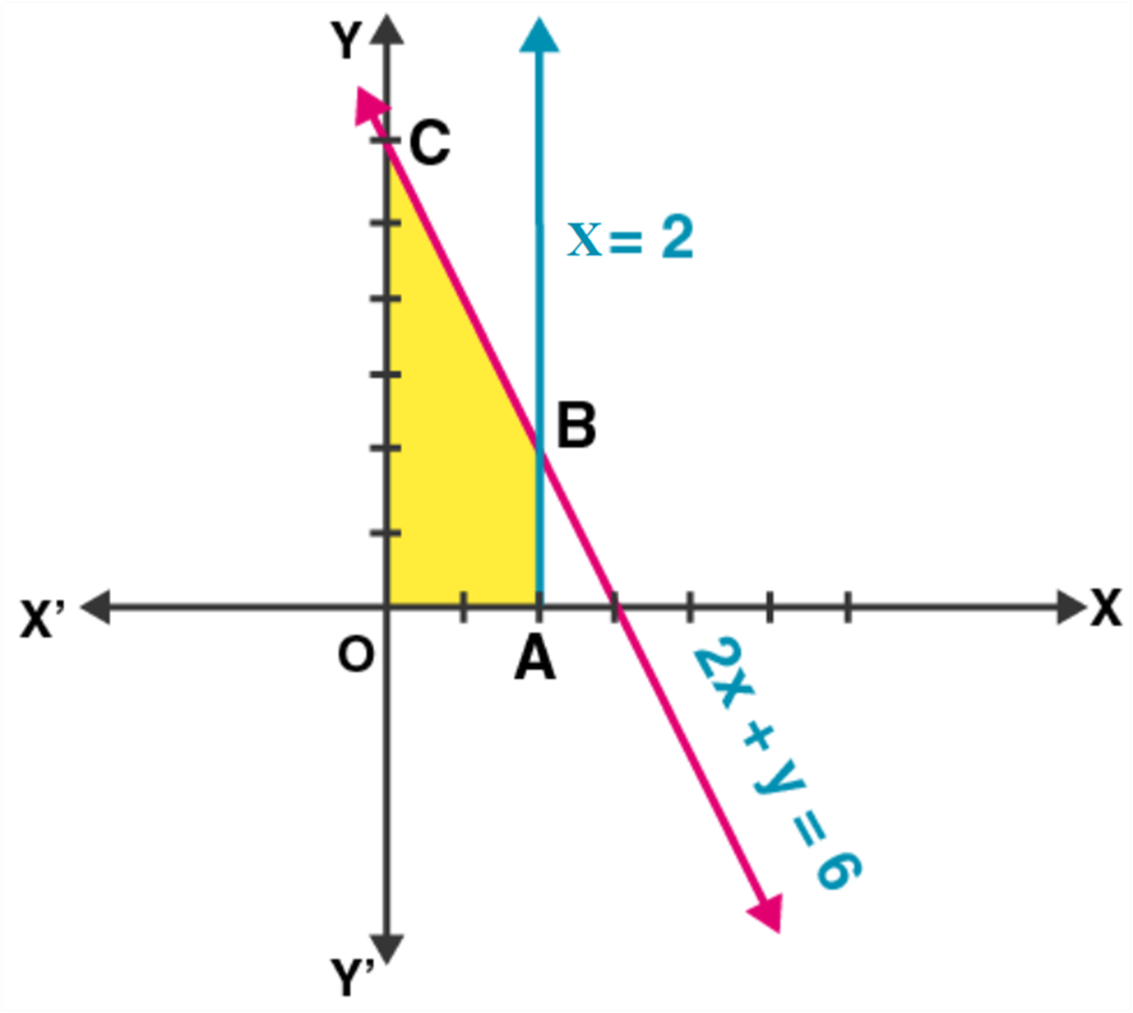
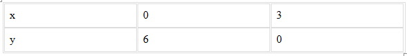
Let 2x + y = 6

Now, plotting all the constrain equations we see that the shaded area OABC is the feasible region determined by the constraints.

The feasible region is bounded. So, the maximum value will occur at a corner point of the feasible region.

Corner points are (0, 0), (2, 0), (2, 2) and (0, 6).

On evaluating the value of Z, we get

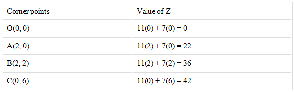
From the above table it’s seen that the maximum value of Z is 42.

Therefore, the maximum value of Z is 42 at (0, 6).

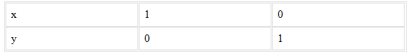
2. Maximize Z = 3x + 4y, subject to the constraints: x + y ≤ 1, x ≥ 0, y ≥ 0.

Solution:

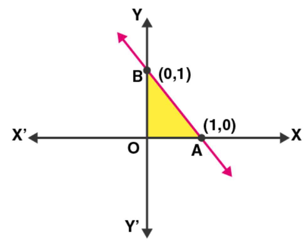
Given: Z = 3x + 4y and the constraints x + y ≤ 1, x ≥ 0,

y ≥ 0

Taking x + y = 1, we have

Now, plotting all the constrain equations we see that the shaded area OAB is the feasible region determined by the constraints.

The area is feasible. So, maximum value will occur at the corner points O(0, 0), A(1, 0), B(0, 1).

On evaluating the value of Z, we get

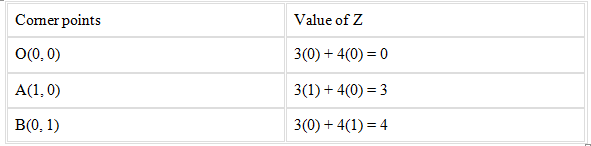
From the above table it’s seen that the maximum value of Z is 4.

Therefore, the maximum value of Z is 4 at (0, 1).

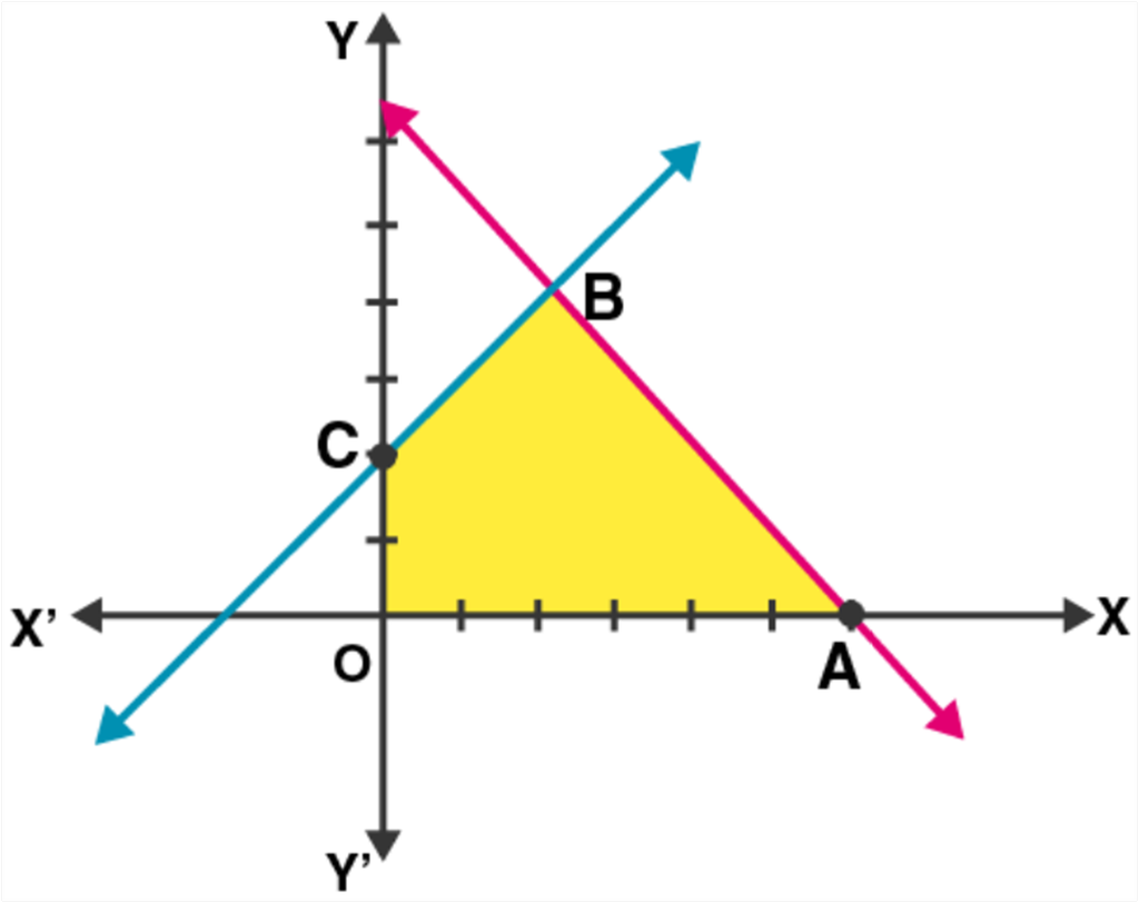
3. Maximize the function Z = 11x + 7y, subject to the constraints: x ≤ 3, y ≤ 2, x ≥ 0, y ≥ 0.

Solution:

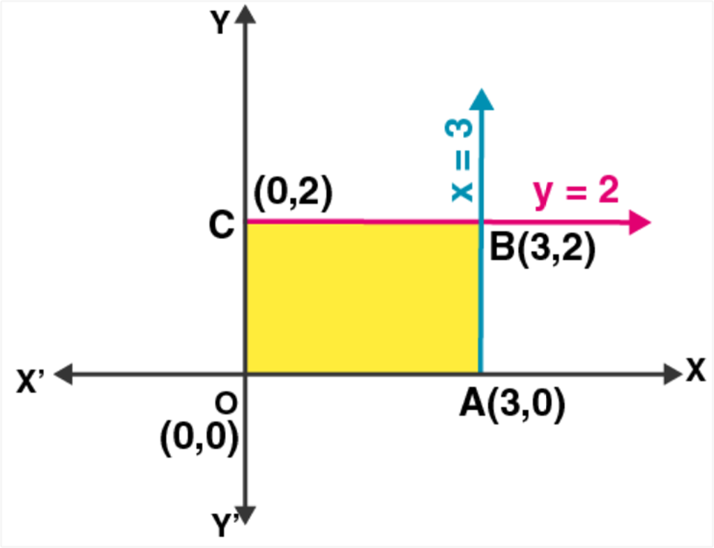
Given: Z = Z = 11x + 7y and the constraints x ≤ 3, y ≤ 2, x ≥ 0, y ≥ 0.

Plotting all the constrain equations we see that the shaded area OABC is the feasible region determined by the constraints.

The feasible region is bounded with four corner points O(0, 0), A(3, 0), B(3, 2) and C(0, 2).

So, the maximum value can occur at any corner.

On evaluating the value of Z, we get

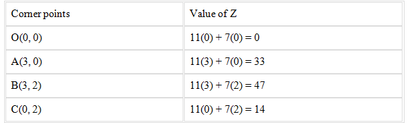
From the above table it’s seen that the maximum value of Z is 47.

Therefore, the maximum value of the function Z is 47 at (3, 2).

4. Minimize Z = 13x – 15y subject to the constraints: x + y ≤ 7, 2x – 3y + 6 ≥ 0, x ≥ 0, y ≥ 0.

Solution:

 

Given: Z = 13x – 15y and the constraints x + y ≤ 7, 2x – 3y + 6 ≥ 0, x ≥ 0, y ≥ 0.

Taking x + y = 7, we have

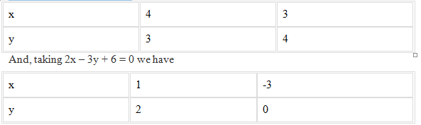
The feasible region is bounded with four corners O(0, 0), A(7, 0), B(3, 4) and C(0, 2).Now, plotting all the constrain equations we see that the shaded area OABC is the feasible region determined by the constraints.

So, the maximum value can occur at any corner.

On evaluating the value of Z, we get

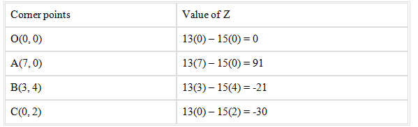
From the above table it’s seen that the minimum value of Z is -30.

Therefore, the minimum value of the function Z is -30 at (0, 2).

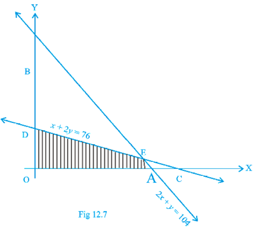
5. Determine the maximum value of Z = 3x + 4y if the feasible region (shaded) for a LPP is shown in Fig. 12.7.

Solution:

As shown in the figure, OAED is the feasible region.

At A, y = 0 in equation 2x + y = 104 we get,

x = 52

This is a corner point A = (52, 0)

At D, x = 0 in equation x + 2y = 76 we get,

y = 38

This is another corner point D = (0, 38)

Now, solving the given equations x + 2y = 76 and 2x + y = 104 we have

2x + 4y = 152

2x + y = 104

(-)___(-)____(-)____

3y = 48 ⇒ y = 16

Using the value of y in the equation, we get

x + 2(16) = 76 ⇒ x = 76 – 32 = 44

So, the corner point E = (44, 16)

On evaluating the maximum value of Z, we get

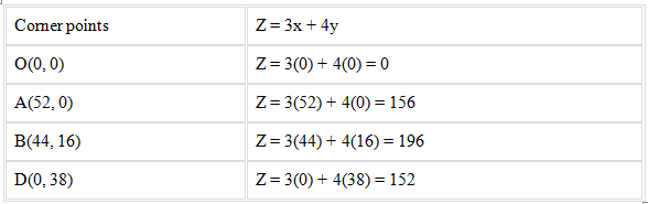
From the above table it’s seen that the maximum value of Z is 196.

Therefore, the maximum value of the function Z is 196 at (44, 16).

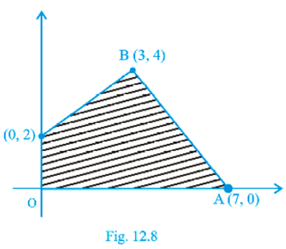
6. Feasible region (shaded) for a LPP is shown in Fig. 12.8. Maximize Z = 5x + 7y.

Solution:

Given: Z = 5x + 7y and feasible region OABC.

The corner points of the feasible region are O(0, 0), A(7, 0), B(3, 4) and C(0, 2).

On evaluating the value of Z, we get

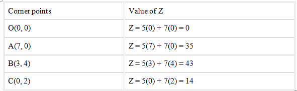
From the above table it’s seen that the maximum value of Z is 43.

Therefore, the maximum value of the function Z is 43 at (3, 4).

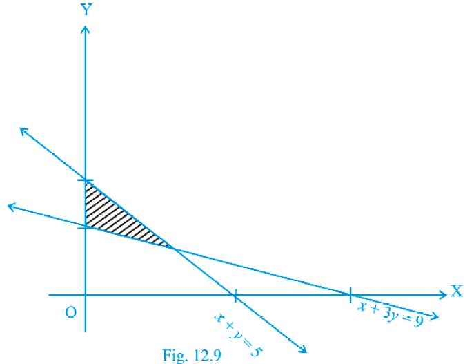
7. The feasible region for a LPP is shown in Fig. 12.9. Find the minimum value of Z = 11x + 7y.

Solution:

In the given figure, it’s seen that the feasible region is ABCA. The corner points are C(0, 3), B(0, 5) and for A, we have to solve equations

x + 3y = 9 and

x + y = 5

(-)_(-)_(-)

2y = 4 ⇒ y = 2

And, putting value of y in the equation we get x = 3

So, the corner point is A(3, 2).

Now, evaluating the value of Z we get

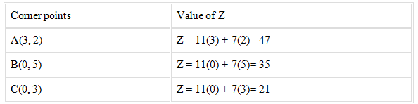
From the above table it’s seen that the minimum value of Z is 21.

Therefore, the minimum value of the function Z is 21 at (0, 3).
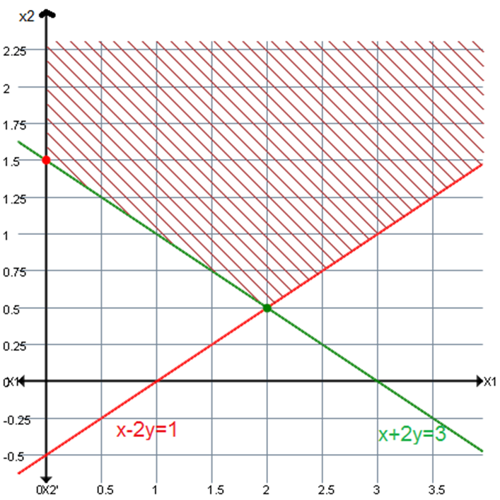
Q8. Find solution using graphical method

max z = 5x₁ + 4x₂

subject to

x₁ - 2 x₂ <= 1

x₁ + 2 x₂ >= 3

and x₁, x₂ >= 0

To draw constraint    x₁ - 2 x₂ ≤1    →  (1)

Let x₁ - 2 x₂ =1
 

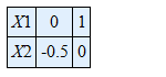
To draw constraint  x₁ + 2 x₂ ≥ 3     →(2)
Let   x₁ + 2 x₂  = 3