 KRISHNA PUBLICATIONS
1. Concept of Continuity and Algebra of continuous functions
- Books Name
- Mathmatics Book Based on NCERT
- Publication
- KRISHNA PUBLICATIONS
- Course
- CBSE Class 12
- Subject
- Mathmatics
Chapter 5
Continuity and Differentiability
Concept of Continuity and Algebra of continuous functions:
Definition-1:
A function f(x) is said to be continuous at x=a if
![]() =f(a)
=f(a)
A function is said to be continuous on the interval [a,b]
if it is continuous at each point in the interval.
Definition-2:
A function f(x) is said to be continuous at a point x = a, in its domain if the following three conditions are satisfied:
- f(a) exists (i.e. the value of f(a) is finite)
- Limx→a f(x) exists (i.e. the right-hand limit = left-hand limit, and both are finite)
- Limx→a f(x) = f(a)
The function f(x) is said to be continuous in the interval I = [x1,x2] if the three conditions mentioned above are satisfied for every point in the interval I.
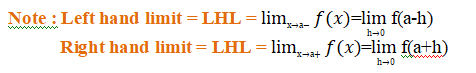
If LHL=RHL ,then limit exists.
If LHL=RHL=f(a), then function is continuous at x = a.
Example 1 Given the graph of f(x), shown below, determine if f(x) is continuous at x=−2, x=0, and x=3.
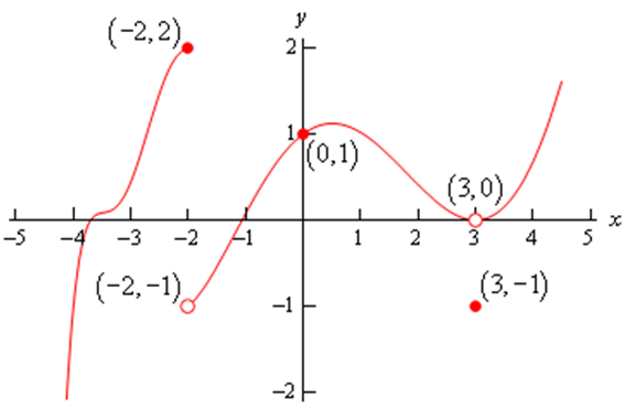
First x=−2.
f(−2)=2 , ![]() doesn't exist.
doesn't exist.
The function value and the limit aren’t the same and so the function is not continuous at this point. This kind of discontinuity in a graph is called a jump discontinuity. Jump discontinuities occur where the graph has a break in it as this graph does and the values of the function to either side of the break are finite (i.e. the function doesn’t go to infinity).
Now x=0
f(0)=1
![]() =1
=1
The function is continuous at this point since the function and limit have the same value.
Finally x=3.
f(3)=−1
![]() =0
=0
The function is not continuous at this point. This kind of discontinuity is called a removable discontinuity. Removable discontinuities are those where there is a hole in the graph as there is in this case.
Discontinuity Conditions:
The function “f” will be discontinuous at x = a in any of the following cases:
- f (a) is not defined.
 And
And  exist but are not equal.
 And
And  exist and are equal but not equal to f (a).
Types of Discontinuity
The four different types of discontinuities are:
- Removable Discontinuity
- Jump Discontinuity
- Infinite Discontinuity
Removable Discontinuity
A function which has well- defined two-sided limits at x = a, but either f(a) is not defined or f(a) is not equal to its limits. ![]()
Example:
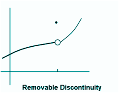
This type of discontinuity can be easily eliminated by redefining the function .
![]()
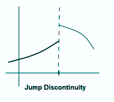
Jump Discontinuity
It is a type of discontinuity, in which the left-hand limit and right-hand limit for a function x = a exists, but they are not equal to each other.![]()
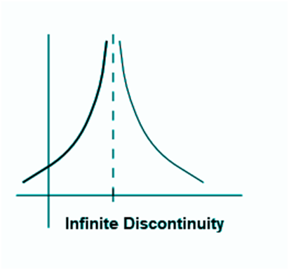
Infinite Discontinuity
The function diverges at x =a to give a discontinuous nature. It means that the function f(a) is not defined. Since the value of the function at x = a does not approach any finite value or tends to infinity, the limit of a function x → a are also not defined.
Example : Discuss the continuity of the function f defined by
f (x) =![]() , x ¹0.
, x ¹0.
Solution Fix any non zero real number c, we have
![]() =
= ![]() =
= ![]() = f( c )
= f( c )
and hence, f is continuous
at every point in the domain of f. Thus f is a continuous function.
Definition -3:
The (ε, δ)-definition of continuity. We recall the definition of continuity: Let f : [a, b] → R and x0 ∈ [a, b]. f is continuous at x0 if for every ε > 0 there exists δ > 0 such that |x − x0| < δ implies |f(x) − f(x![]() )| < ε. We sometimes indicate that the δ may depend on ε by writing δ(ε).
)| < ε. We sometimes indicate that the δ may depend on ε by writing δ(ε).
Example:
The function defined by f (x) = √x is continuous.
Proof:
Given ε > 0 we must show that |√x - √p| < ε provided that x, p are close enough.
Now |√x - √p| = |x - p|/|√x + √p| < |x - p| /√p and so choosing δ = ε/√p will do.
Definition
If f and g are functions from R to R, we define the function f + g by (f + g)(x) = f (x) + g(x) for all x in R.
Similarly we may define the difference, product and quotient of functions.
Theorem
If f and g are continuous a point p of R, then so are f + g, f - g, f.g and (provided g(p) ≠ 0) f /g .
Proof
This follows directly from the corresponding arithmetic properties of sequences.
For example: to prove that f + g is continuous at p ∈ R
Suppose (xn)→ p. We are told that (f (xn))→ f (p) and (g(xn))→ g(p) and we must prove that (f + g)(xn))→ (f + g)(p).
But the LHS of this expression is f (xn) + g(xn) and the RHS is f (p) + g(p) and so the result follows from the arithmetic properties of sequences
Theorem
The composite of continuous functions is continuous.
Proof
Suppose f: R→ R and g: R→ R. Then the composition g  f is defined by g f (x) = g(f (x)).
We assume that f is continuous at p and that g is continuous at f (p). So suppose that (xi)→ p. Then (f (xi))→ f (p) and then (g(f (xi)))→ g(f (p)) which is what we need.
Examples
- Clearly the identity function which x ↦ x is continuous.
Hence, using the above, any polynomial function is continuous and hence any rational function (a ratio of polynomial functions) is continuous at any point where the denominator is non-zero. - We will prove later that functions like √x, sinx, cosx, exp(x), logx, ... are continuous. It follows that , for example sin2(x + 5), exp(-x2), √(1 + x4), ... are continuous since they are made by composing continuous functions.
![]()
Hence, the function f(x) is continuous at x =0.
Algebra of continuous functions:
Theorem : Suppose f and g be two real functions continuous at a real number c.
Then
(1) f + g is continuous at x = c.
(2) f – g is continuous at x = c.
(3) f . g is continuous at x = c.
(4) f/g is continuous at x = c, (provided g(c) ¹0).
(5) the algebraic operations between two functions are also continuous.
(6) f(g(x)) and g(f(x)) are continuous at x = a (Composite Function is continuous)
(7) Trigonometric Function is Continuous
(8) Exponential Function is Continuous
(9) Logarithm function is continuous .
(10) Polynomial Function is continuous.
(11) Modulus Function is Continuous.
(12) All rational functions are continuous.
Proof: (1) Given,
limx→a f(x) = f(a)
limx→ a g(x) = g(a)
Now as per the theorem,
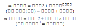
limx → a (f+g)(x) ⇒ lim x → c [f(x) + g(x)]
⇒ limx → c f(x) + limx → c g(x)
⇒ f(a) + g(a)
⇒ (f + g)(a)
Therefore,
limx → a (f+g)(x) = (f + g)(c)
Hence, f+g is continuous at x = a.
(3)
Proof: Given,
limx→a f(x) = f(a)
limx→ a g(x) = g(a)
So, the limit of product of two functions, f and g at x is given by:
limx → a (f . g)(x) ⇒ lim x → c [f(x) . g(x)]
⇒ limx → c f(x) . limx → c g(x)
⇒ f(a) . g(a)
⇒ (f . g)(a)
Therefore,
limx → a (f . g)(x) = (f . g)(c)
Hence, f . g is continuous at x = a.
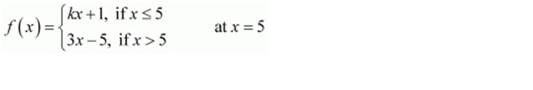
Question :Find the values of k so that the function f is continuous at the indicated point.
ANSWER:
The given function f is
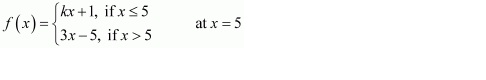
The given function f is continuous at x = 5, if f is defined at x = 5 and if the value of f at x = 5 equals the limit of f at x = 5
It is evident that f is defined at x = 5 and f(5)=kx+1=5k+1
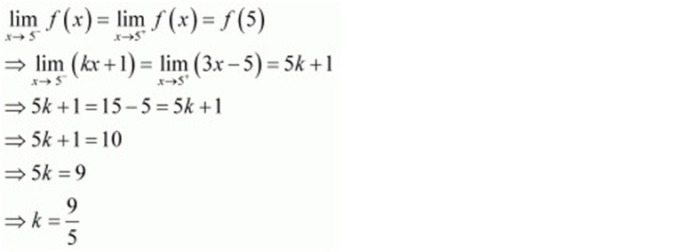
Therefore, the required value of 9/5.
Problem:
Prove that the function defined by f(x) = | cos x | is a continuous function.
Solution: Given, f(x) = |cos x|
f(x) is the real function for all real numbers ‘x’ and the domain of f(x) is the real number
Let g(x) = cos x and h(x) = |x|
g(x) and h(x) are cosine functions and modulus functions are continuous for all real numbers.
Now,
(goh) (x) = g (h(x)) = g(|x|) = cos |x| is a composite function, hence is a continuous function. But it is not equal to f(x).
Again,
(hog) (x) = h(g(x)) = g(cos x) = |cos x| = f(x) [Given]
Hence,
f(x) = |cos x| = hog (x) is a composition function of two continuous functions. Therefore, it is also a continuous function.
Continuity in open interval (a, b)
f(x) will be continuous in the open interval (a,b) if at any point in the given interval the function is continuous.
Continuity in closed interval [a, b]
A function f(x) is said to be continuous in the closed interval [a,b] if it satisfies the following three conditions.
1) f(x) is be continuous in the open interval (a, b)
2) f(x) is continuous at the point a from right i.e.![]()
3) f(x) is continuous at the point b from left i.e. ![]()
2. Concept of Differentiability and Algebra of derivatives
- Books Name
- Mathmatics Book Based on NCERT
- Publication
- KRISHNA PUBLICATIONS
- Course
- CBSE Class 12
- Subject
- Mathmatics
Concept of Differentiability and Algebra of derivatives :
Differentiability:
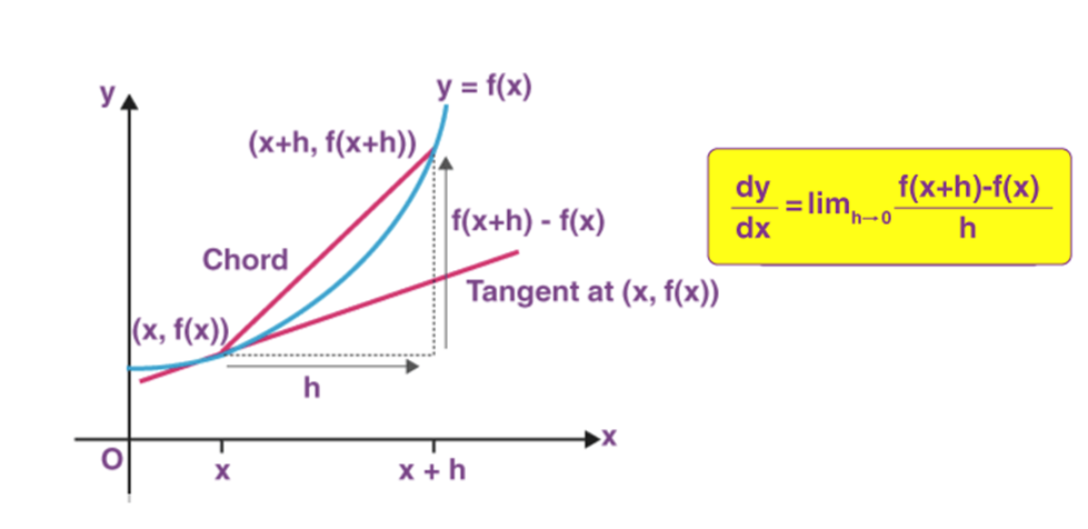
A function is differentiable at a point when there's a defined derivative at that point. This means that the slope of the tangent line of the points from the left is approaching the same value as the slope of the tangent of the points from the right.
The computation of the slope of a tangent line, the instantaneous rate of change of a function, and the instantaneous velocity of an object at x=a all required us to compute the following limit.
A function f : U -> R, defined on an open set UÍR, is said to be differentiable at aÎU, if the derivative
exists. This implies that the function is continuous at a.
This function f is said to be differentiable on U if it is differentiable at every point of U. In this case, the derivative of f is thus a function from U into R.
A continuous function is not necessarily differentiable, but a differentiable function is necessarily continuous (at every point where it is differentiable)
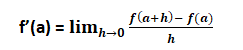
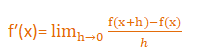
The derivative of f(x) with respect to x is the function f′(x) and is defined as,
Derivative of f at c is denoted by f ¢(c) or ![]()
![]()
wherever the limit exists is defined to be the derivative of f.
The derivative of f is denoted by f '(x) or ![]()
The process of finding derivative of a function is called differentiation.
Algebra of derivatives:
Properties: Let u=u(x), v=v(x) and w=w(x) be three differentiable function.
(1) (u ± v)¢ = u¢ ± v (Sum Rule of Differentiation)
(2) (uv)¢ = u¢v + uv¢ (Leibnitz or product rule)
(3)![]() ,wherever v ¹ 0 (Quotient rule).
,wherever v ¹ 0 (Quotient rule).
(4) (uvw)’ = uv w’ + uwv’ + vw u’
Theorem : If a function f is differentiable at a point c, then it is also continuous at that
point.
Solution :
Since f is differentiable at c, we have
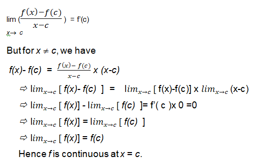
Corollary : Every differentiable function is continuous but vice versa is not true.
we have seen that the function defined by f (x) = | x| is a continuous function.
Consider the
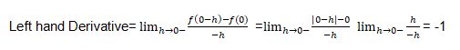
![]()
Since the above left and right hand Derivative at 0 are not equal,
Limit does not exist and hence f is not differentiable at 0.
Thus every continuous function is not differentiable function.
3. Derivatives of composite functions
- Books Name
- Mathmatics Book Based on NCERT
- Publication
- KRISHNA PUBLICATIONS
- Course
- CBSE Class 12
- Subject
- Mathmatics
Derivatives of composite functions
Theorem: (Chain Rule) Let f be a real valued function which is a composite of two
functions u and v; i.e., f = v o u. Suppose t = u(x) and if both 
we have ![]()
Example: Find the derivative of the function given by f (x) = sin (x2).
Ans:
Let
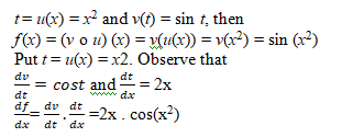
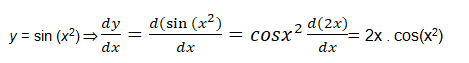
Alternatively, We can also directly proceed as follows:
Example :
Find the derivative of sin x – cos x.
Solution:
Given function is: sin x – cos x
Let f(x) = sin x and g(x) = cos x
Using the difference rule of differentiation,
d/dx [f(x) – g(x)] = d/dx f(x) – d/dx g(x)
d/dx (sin x – cos x) = d/dx (sin x) – d/dx (cos x)
= cos x – (-sin x)
= cos x + sin x
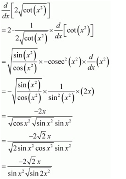
Problem:
Differentiate the functions with respect to x.
![]()
Ans;
10. Mean Value Theorem
- Books Name
- Mathmatics Book Based on NCERT
- Publication
- KRISHNA PUBLICATIONS
- Course
- CBSE Class 12
- Subject
- Mathmatics
Mean Value Theorem:
Rolle’s Theorem which states that:
Rolle’s Mean Value Theorem
If a function f is defined in the closed interval [a, b] in such a way that it satisfies the following conditions.
i) The function f is continuous on the closed interval [a, b]
ii)The function f is differentiable on the open interval (a, b)
iii) and f (a) = f (b) ,
then there exists at least one value of x=cÎ (a, b) such that f'(c) = 0.
Geometric interpretation of Rolle’s Theorem
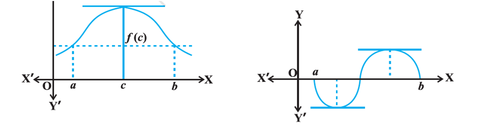
Observe what happens to the slope of the tangent to the curve at various points
between a and b. In each of the graphs, the slope becomes zero at least at one point.
That is precisely the claim of the Rolle’s theorem as the slope of the tangent at any
point on the graph of y = f (x) is nothing but the derivative of f (x) at that point.
Lagrange’s Mean Value Theorem (LMVT)
Lagrange’s Mean Value Theorem or First Mean Value theorem states that a function f is defined in the closed interval [a, b], it satisfies the following conditions:
- The function f is always continuous in the closed interval [a, b]
- The function is always differentiable in the open interval (a, b)
And there exists at least one value x = cÎ (a,b) such that,
[f(b)–f(a)]/ (b-a) = f’ (c)
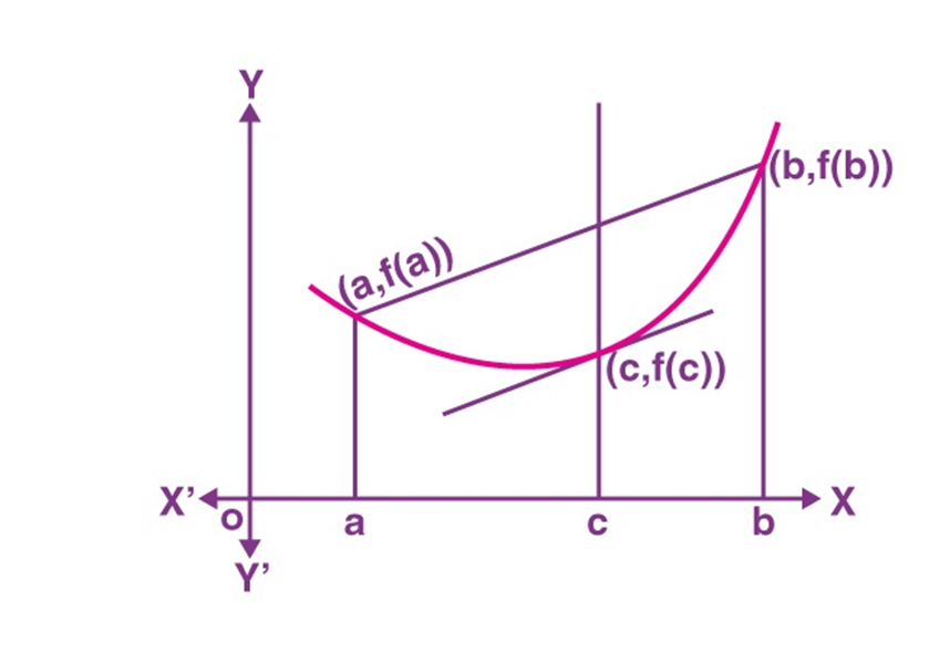
Geometrical Representation of Lagrange’s Mean Value Theorem
The graph given below the curve y = f(x) is The function f is
i) continuous on the closed interval [a, b]
ii)The function f is differentiable on the open interval (a, b)
then, According to the Lagrange Mean Value Theorem,
Any function that is continuous on [a,b] and also differentiable on (a,b) has some in the interval (a,b) such that the secant joining the interval's ends is parallel to the tangent at point C.
f ’(c) = [ f (b) –f (a)]/(b-a)
Example:
Verify Mean Value Theorem for the function f(x) = x2 – 4x – 3 in the interval [a, b], where a = 1 and b = 4.
Solution:
Given,
f(x) = x2 – 4x – 3
f'(x) = 2x – 4
a = 1 and b = 4 (given)
f(a) = f(1) = (1)2 – 4(1) – 3 = 1 – 4 – 3 = -6
f(b) = f(4) = (4)2 – 4(4) – 3 = -3
Now,
[f(b) – f(a)]/ (b – a) = (-3 + 6)/(4 – 1) = 3/3 = 1
As per the Lagrange’s mean value theorem statement, there is a point c ∈ (1, 4) such that
f'(c) = [f(b) – f(a)]/ (b – a),
i.e. f'(c) = 1.
2c – 4 = 1
2c = 5
c = 5/2 ∈ (1, 4)
Verification: f'(c) = 2(5/2) – 4 = 5 – 4 = 1
Hence, verified the mean value theorem.
Example:
Verify Rolle’s theorem for the function y = x2 + 2, a = –2 and b = 2.
Solution:
From the definition of Rolle’s theorem, the function y = x2 + 2 is continuous in [– 2, 2] and differentiable in (– 2, 2).
From the given,
f(x) = x2 + 2
f(-2) = (-2)2 + 2 = 4 + 2 = 6
f(2) = (2)2 + 2 = 4 + 2= 6
Thus, f(– 2) = f( 2) = 6
Hence, the value of f(x) at –2 and 2 coincide.
Now, f'(x) = 2x
Rolle’s theorem states that there is a point c ∈ (– 2, 2) such that f′(c) = 0.
At c = 0, f′(c) = 2(0) = 0, where c = 0 ∈ (– 2, 2)
Hence verified.
4. Derivatives of implicit functions
- Books Name
- Mathmatics Book Based on NCERT
- Publication
- KRISHNA PUBLICATIONS
- Course
- CBSE Class 12
- Subject
- Mathmatics
Derivatives of implicit functions:
Implicit functions are functions where a specific variable cannot be expressed as a function of the other variable. A function that depends on more than one variable.
we’ll adopt the following procedure:
- Given an implicit function with the dependent variable y and the independent variable x (or the other way around).
- Differentiate the entire equation with respect to the independent variable (it could be x or y).
- After differentiating, we need to apply the chain rule of differentiation.
- Solve the resultant equation for dy/dx (or dx/dy likewise) or differentiate again if the higher-order derivatives are needed.
“Some function of y and x equals to something else”. Knowing x does not help us compute y directly.
Example, x2 + y2 = r2 (Implicit function)
Differentiate with respect to x:
d(x2) /dx + d(y2)/ dx = d(r2) / dx
Solve each term:
Using Power Rule: d(x2) / dx = 2x
Using Chain Rule : d(y2)/ dx = 2y dydx
r2 is a constant, so its derivative is 0: d(r2)/ dx = 0
Which gives us:
2x + 2y dy/dx = 0
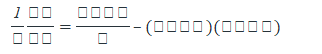
Collect all the dy/dx on one side
y dy/dx = −x
Solve for dy/dx:
dy/dx = −xy
Example . Find dy/dx if x2y3 − xy = 10.
Solution:
2xy3 + x2. 3y2 . dy/dx – y – x . dy/dx = 0
(3x2y2 – x ) . dy/dx = y – 2xy3
dy/dx = (y – 2xy3) / (3x2y2 – x)
Example . Find dy/dx if y = sinx + cosy
Solution:
y – cosy = sinx
dy/dx + siny. dy/dx = cosx
dy/dx = cosx / (1 + siny)
Example . Find the slope of the tangent line to the curve x2+ y2= 25 at the point (3,−4).
Solution:
Note that the slope of the tangent line to a curve is the derivative, differentiate implicitly with respect to x, which yields,
2x + 2y. dy/dx = 0
dy/dx = -x/y
Hence, at (3,−4), y′ = −3/−4 = 3/4, and the tangent line has slope 3/4 at the point (3,−4).
5. Derivatives of inverse trigonometric functions
- Books Name
- Mathmatics Book Based on NCERT
- Publication
- KRISHNA PUBLICATIONS
- Course
- CBSE Class 12
- Subject
- Mathmatics
Derivatives of inverse trigonometric functions:
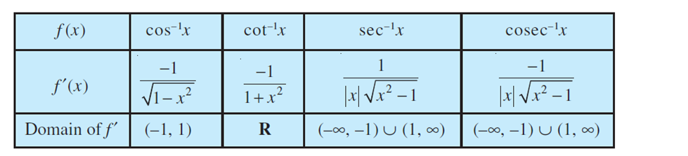
Inverse of sin x = arcsin(x) or
Let us now find the derivative of Inverse trigonometric function
Example: Find the derivative of a function ![]()
Solution: Given
![]()
Differentiating the above equation w.r.t. x, we have:
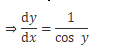
Putting the value of y form (i), we get
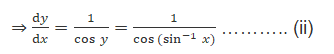
From equation (ii), we can see that the value of cos y cannot be equal to 0, as the function would become undefined ![]()
i. e.![]()
From (i) we have ![]()
![]()
Using property of trigonometric function,
![]()
![]()
Now putting the value of (iii) in (ii), we have ![]()
Therefore, the Derivative of Inverse sine function is ![]()
Example:Find the derivative of a function
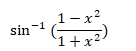
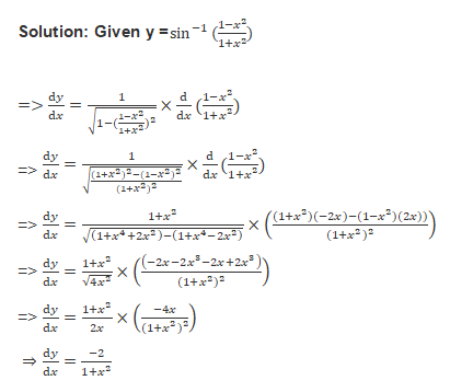
Problem: y = cot-1(1/x2)
Solution:
As we are solving the above three problem in the same way this problem will solve
By using chain rule,
y’ = (cot-1(1 / x2))’
= { – 1 / (1 + (1 / x2))2 } . (1 / x2)’
= { – 1 / (1 + (1 / x4)) . (-2x-3)
= 2x4 / (x4 + 1)x3
Example: Solve f(x) = tan-1(x) Using first Principle.
Solution:
For solving and finding tan-1x, we have to remember some formulae, listed below.
- limh->0 {f(x + h) – f(x)} / h
- tan-1(θ/θ) = 1
- tan-1x – tan-1y = tan-1[(x – y) / (1 + xy)]
f(x) = tan-1x
f(x + h) = tan-1(x + h)
Apply 1st formula
limh->0 {tan-1(x + h) – tan-1x } / h
Now Apply 3rd formula
limh->0 tan-1[(x – h – x) / (1 + (x + h)x] / h
limh->0 tan-1[(h / (1 + x2 + xh ] / h . [(1 + x2 + xh) / (1 + x2 + xh)]
limh->0 tan-1 {h / 1 + x2 + xh} / {h / 1 + x2 + xh} . limh->0 1 / 1 + x2 + xh
Now we made the solution like so that we apply the 2nd formula
= 1 . 1 / (1 + x2 + x . 0)
= 1 / (1 + x2)
6. Derivatives of Exponential and Logarithmic Functions
- Books Name
- Mathmatics Book Based on NCERT
- Publication
- KRISHNA PUBLICATIONS
- Course
- CBSE Class 12
- Subject
- Mathmatics
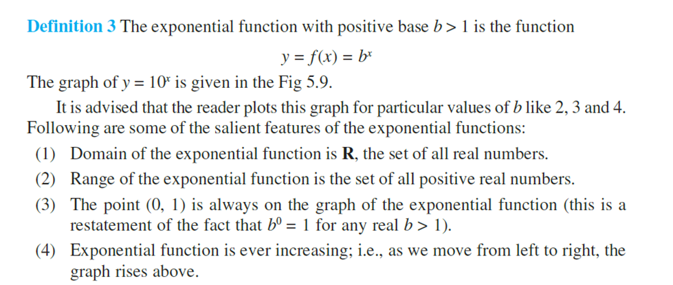
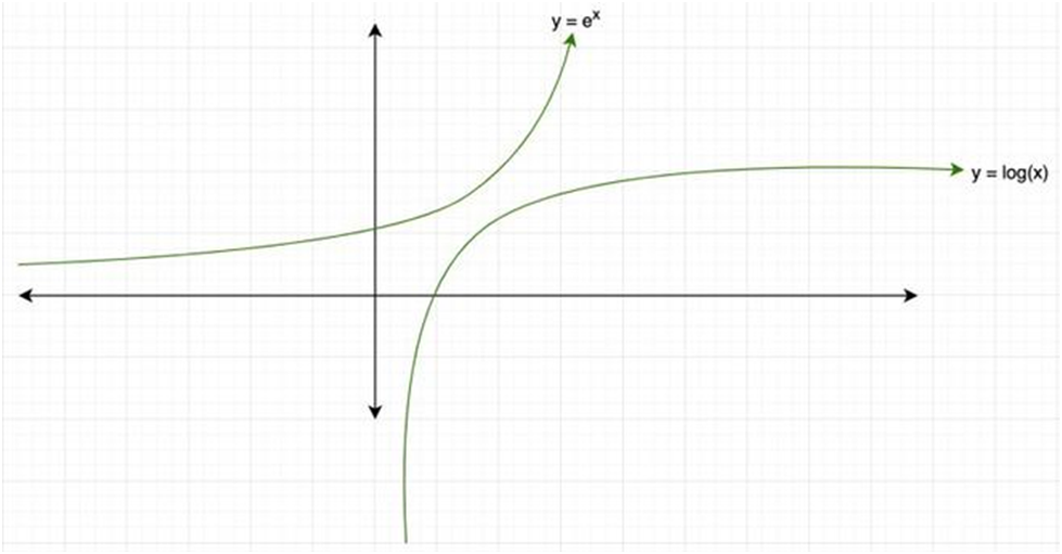
Derivatives of Exponential and Logarithmic Functions:
7. Logarithmic Differentiation
- Books Name
- Mathmatics Book Based on NCERT
- Publication
- KRISHNA PUBLICATIONS
- Course
- CBSE Class 12
- Subject
- Mathmatics
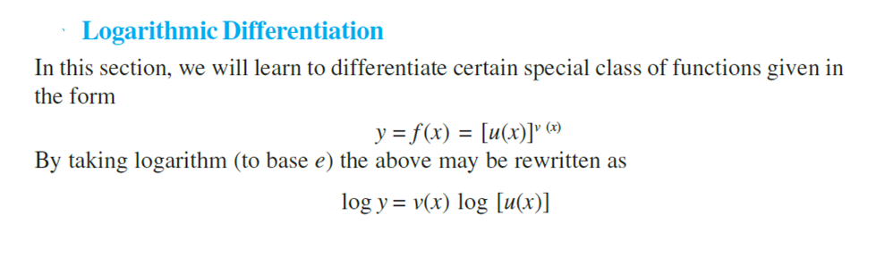
Logarithmic Differentiation:
If function to the power function or function to the power variable or variable to the power function or variable to the power variable ,then apply logarithm.
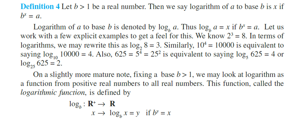
The derivative of ex w.r.t. x = d/dx (ex) = ex
The derivative of log x w.r.t. x = d/dx (log x) = 1/x
Now this last limit  is exactly the definition of above derivative f'(x) at x = 0, i.e f'(0). Therefore, the derivative becomes,
f'(x) = bxf'(0) = bx
So, in case of natural exponential functions, f(x) = ex
Note: In general exponential cases, for example, y = bx, where b is a real number. The derivative for this kind of function is
![]()
Question: Differentiate f(x) = 4ex – 5x
Answer:
The derivation of ex will remain ex, the derivative of 5x will become 5xln(5) as explained above.
Therefore, f'(x) = 4ex – 5xln(x)
Question : Find the value of F'(x) at x=0 when f(x) = 7x + 2ex
Answer:
Differentiating: f'(x) = 7xln(7) + 2ex
at x=0, f'(0) = 70ln(7) + 2e0
= ln(7) + 2
= 3.945
Question: d/dx(xx) = xx(1+ln x)
Question: Find the value of
if y = 2x{cos x}.
Solution: Given the function y = 2x{cos x}
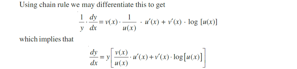
Taking logarithm of both the sides, we get
log y = log(2x{cos x})
Now, differentiating both the sides w.r.t by using the chain rule we get,
8. Derivatives of Functions in Parametric Forms
- Books Name
- Mathmatics Book Based on NCERT
- Publication
- KRISHNA PUBLICATIONS
- Course
- CBSE Class 12
- Subject
- Mathmatics
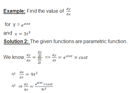
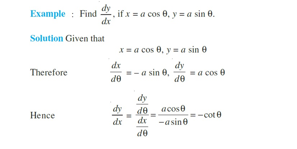
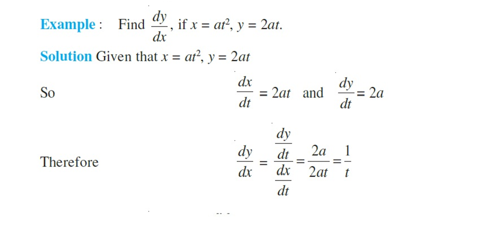
Derivatives of Functions in Parametric Forms:
A parametric derivative is a derivative of a dependent variable with respect to another dependent variable that is taken when both variables depend on an independent third variable, usually thought of as "time" (that is, when the dependent variables are x and y and are given by parametric equations in t).
More precisely, a relation expressed between two variables x and y in the form
x = f (t), y = g(t) is said to be parametric form with t as a parameter.
or

This is the required solution.
9. Second Order Derivative
- Books Name
- Mathmatics Book Based on NCERT
- Publication
- KRISHNA PUBLICATIONS
- Course
- CBSE Class 12
- Subject
- Mathmatics
Second Order Derivative:
The first-order derivative at a given point gives us the information about the slope of the tangent at that point or the instantaneous rate of change of a function at that point. Second-Order Derivative gives us the idea of the shape of the graph of a given function. The second derivative of a function f(x) is usually denoted as f”(x). It is also denoted by D2y or y2 or y” if y = f(x).
Let y = f(x)
Then, dy/dx = f'(x)
If f'(x) is differentiable, we may differentiate (1) again w.r.t x. Then, the left-hand side becomes d/dx(dy/dx) which is called the second order derivative of y w.r.t x.
Example: Find d2y/dx2, if y = x3?
Solution:
Given that, y = x3
Then, first derivative will be
dy/dx = d/dx (x3) = 3x2
Again, we will differentiate further to find its
second derivative,
Therefore, d2y/dx2 = d/dx (dy/dx)
= d/dx (3x2)
= 6x
Example : Find d2y/dx2, if y = Asinx + Bcosx, Where A and B are constants?
Solution:
Given that, y = Asinx + Bcosx
Then, first derivative will be
dy/dx = d/dx (Asinx + Bcosx)
= A d/dx (sinx) + B d/dx (cosx)
= A(cosx) + B(-sinx)
= Acosx – Bsinx
Again, we will differentiate further to find its second derivative,
d2y/dx2 = d/dx (dy/dx)
= d/dx (Acosx – Bsinx)
= A d/dx (cosx) – B d/dx (sinx)
= A(-sinx) – B(cosx)
= -Asinx – Bcosx
= -(Asinx + Bcosx)
= -y
Example: If x = t + cost, y = sint, find the second derivative.
Solution:
Given that, x = t + cost and y = sint
First Derivative,
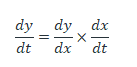
dy/dx = (dy/dt) / (dx/dt)
= (d/dt (sint)) / (d/dt (t + cost))
= (cost) / (1 – sint) ……. (1)
Second Derivative,
d2y / dx2 = d/dx (dy/dx)
= d/dx (cost / 1 – sint) …….. (from eq.(1))
= d/dt (cost / 1 – sint) / (dx/dt) ………(chain rule)
= ((1 – sint) (-sint) – cost(-cost)) / (1 – sint)2 / (dx/dt) …. (quotient rule)
= (-sint + sin2t + cos2t) / (1 – sint)2 / (1 – sint)
= (-sint + 1) / (1 – sint)3
= 1 / (1 – sint)2