Chapter 15

Statistics

Statistics : Measures of Dispersion:

A measure of central tendency gives us a rough idea where data points are centred.

the measures of central tendency are not sufficient to give complete information about a given data. Variability is another factor which is required to be studied under statistics. Like ‘measures of central tendency’ we want to have a single number to describe variability. This single number is called a ‘measure of dispersion’.

In statistics, dispersion (also called variability, scatter, or spread) is the extent to which a distribution is stretched or squeezed. Common examples of measures of statistical dispersion are the variance, standard deviation, and interquartile range. For instance, when the variance of data in a set is large, the data is widely scattered. On the other hand, when the variance is Small, the data in the set is clustered.

A measure of statistical dispersion is a nonnegative real number that is zero if all the data are the same and increases as the data become more diverse.

Most measures of dispersion have the same units as the quantity being measured. In other words, if the measurements are in metres or seconds, so is the measure of dispersion.

Dispersion is contrasted with location or central tendency, and together they are the most used properties of distributions.

A measure of dispersion indicates the scattering of data. It explains the disparity of data from one another, delivering a precise view of their distribution. The measure of dispersion displays and gives us an idea about the variation and the central value of an individual item.

OR

the measures of dispersion help to interpret the variability of data i.e. to know how much homogenous or heterogeneous the data is. In simple terms, it shows how squeezed or scattered the variable is.

Measures of dispersion are vital because they can show you the within a specific sample, or group of people. When it comes to samples, that dispersion is important because it determines the margin of error you'll have when making inferences about measures of central tendency, like averages.

The variation can be measured in different numerical measures, namely:

(i) Range: It is the simplest method of measurement of dispersion and defines the difference between the largest and the smallest item in a given distribution. If Y max and Y min are the two ultimate items, then

Range = Y max – Y min

(ii) Quartile deviation: It is known as semi-interquartile range, i.e., half of the difference between the upper quartile and lower quartile. The first quartile is derived as Q, the middle digit Q1 connects the least number with the median of the data. The median of a data set is the (Q2) second quartile. Lastly, the number connecting the largest number and the median is the third quartile (Q3). Quartile deviation can be calculated by

Q = ½ × (Q3 – Q1)

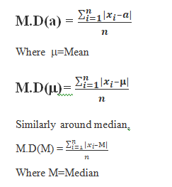
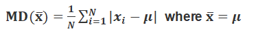
(iii) Mean deviation: Mean deviation is the arithmetic mean (average) of deviations  ⎜MD ⎜of observations from a central value (mean or median).

Mean deviation can be evaluated by using the formula: 

Thus mean deviation about a central value ‘A’ is the mean of the absolute values of the deviations of the observations

from ‘A’. The mean deviation from ‘a’ is denoted as M.D. (A).

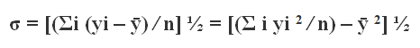
(iv) Standard deviation: Standard deviation is the square root of the arithmetic average of the square of the deviations measured from the mean. The standard deviation is given as,

Mean

The average of the given set of data is computed by dividing the total number of numbers by the sum of the given numbers.

Mean = (Sum of all observations/Total number of observations)

Mean for Ungrouped Data

Example:

There are 20 pupils in a class, and their grades are 88, 82, 88, 85, 84, 80, 81, 82, 83, 85, 84, 74, 75, 76, 89, 90, 89, 80, 82, and 83.

The mean is the sum of the percentages obtained

= [88 + 82 + 88 + 85 + 84 + 80 + 81 + 82 + 83 + 85 + 84 + 74 + 75 + 76 + 89 + 90 + 89 + 80 + 82 + 83] /20 = 1660/20 = 83 %

Mean for Grouped Data

In statistics, the mean, or arithmetic mean, of a group of numbers is the sum of the numbers divided by the number of numbers in the group. The mean is a measure of the central tendency of a group of numbers.

When dealing with grouped data, the mean is calculated by first finding the midpoint of each group, then finding the sum of the numbers in each group, and finally dividing the sum by the number of groups.

Chapter 16

Probability

Probability and Random experiments:

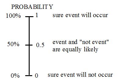
A probability is simply a number between 0 and 1 that measures the uncertainty of a particular event.

Although many events are uncertain, we possess different degrees of belief about the truth of an uncertain event.

Many events cannot be predicted with total certainty. We can predict only the chance of an event to occur i.e. how likely they are to happen, using it. Probability can range in from 0 to 1, where 0 means the event to be an impossible one and 1 indicates a certain event.

OR

Probability is the branch of mathematics concerning numerical descriptions of how likely an event is to occur, or how likely it is that a proposition is true. The probability of an event is a number between 0 and 1, where, roughly speaking, 0 indicates impossibility of the event and 1 indicates certainty.

For example, most of us are pretty certain of the statement "the sun will rise tomorrow", and pretty sure that the statement "the moon is made of green cheese" is false.

For example, when we toss a coin, either we get Head OR Tail, only two possible outcomes are possible (H, T). But if we toss two coins in the air, there could be three possibilities of events to occur, such as both the coins show heads or both show tails or one shows heads and one tail, i.e.(H, H), (H, T),(T, T).

The Classical view of a Probability

Suppose that we observe some phenomena (say, the rolls of two dice) where the outcome is random. Suppose we can write down the list of all possible outcomes, and we believe that each outcome in the list has the same probability. Then the probability of each outcome will be

P(outcome)=1/(number of outcomes)

The Frequency View of a Probability

The classical view of probability is helpful only when we can construct a list of outcomes of the experiment in such a way where the outcomes are equally likely.

The frequency interpretation of probability can be used in cases where outcomes are equally likely or not equally likely.

This view of probability is appropriate in the situation where we are able to repeat the random experiment many times under the same conditions.

An Experiment is defined as a process whose result is well defiened

Two types of Experiment:

1. Deterministic Experiment
2. Random Experiment

Deterministic Experiment:

It is an Experiment whose outcomes can be predicted with certainty under identical conditions.

Example: When we heat water it will evaporate

Example: When we toss a two headed coin we will get a head.

Random Experiment

It is an experiment whose all possible outcomes are known but it is not possible to predict the exact outcomes in advance.

Or

A random experiment is a mechanism that produces a definite outcome that  cannot be predicted with certainty.

Example: An unbiased coin is tossed.

Example: A die is rolled.

Random Experiment always satisfies the following two conditions:

1. It has more than one possible outcomes
2. It is not possible to predict the outcome in advance.

The two possible outcomes are getting a head or a tail. The outcome of this experiment cannot be predicted before it has been performed. Furthermore, it can be conducted many times under the same conditions. Thus, tossing a coin is an example of a random experiment.

Outcome: A possible result of a random experiment is called its outcome.

Mean deviation, range, variance and standard deviation of grouped and ungrouped data:

Range of Ungrouped Data

We know now that range is the difference between the maximum and minimum value. Hence for ungrouped data, we arrange the series in ascending or descending order. This helps us to select the highest and lowest values in the distribution. Henceforth, we simply subtract the minimum value from the maximum value.

Example :

The marks of a student in 5 tests of the chapter statistics are(out of 20)- 11, 14, 16, 13 and 18.

Arranging them in ascending order- 18, 16, 14, 13 and 11. The range of the data is given as- 18-11=7.

Range= Maximum value – Minimum value

Mean Deviation for Ungrouped Data

Mean deviation measures the dispersion of data about a measure of central tendency. This measure of central tendency is generally median or mean. How to calculate mean and median for individual distribution series.

Calculating Mean and Median

For calculation of median, we first arrange the data in ascending or descending order(generally ascending order). Further, we count the number of observations which is denoted by n. Now depending on whether n is even or odd, the further calculation is bifurcated as:

• If n is an odd number then the value of (n+1)/2^th item is the median.
• If n is an even number then median is given as: [ value of (n+1)/2^th item + value of (n/2 +1)^th item]÷2 

Mean is simply calculated as the ration of summation of observations to the number of observations.

Mean= Sum of observations/number of observations

Steps to Calculate the Mean Deviation for Ungrouped data

To calculate the mean deviation for ungrouped data, the following steps are followed:

Let the set of data consist of  observations.

Step i) The measure of central tendency about which mean deviation is to be found out is calculated. Let a be assumed mean.

Step ii) Calculate the absolute deviation of each observation from the measure of central tendency calculated in step (i) i.e.,

Step iii) Evaluate the mean of all the absolute deviations. This gives the mean absolute deviation (M.D) about ‘a‘ for ungrouped data i.e.,

In case the measure of central tendency is mean the above equation can be rewritten as:

Mean Deviation Formulas for Grouped Data:

Mean deviation for grouped data We know that data can be grouped into

two ways :

(a) Discrete frequency distribution,

(b) Continuous frequency distribution.

Let us discuss the method of finding mean deviation for both types of the data.

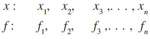
(a) Discrete frequency distribution Let the given data consist of n distinct values

x1, x2, ..., xn occurring with frequencies f1, f2 , ..., fn respectively. This data can be

represented in the tabular form as given below, and is called discrete frequency

distribution:

x : x1  x2  x3 ... xn

f : f1   f2     f3  ... fn

(i) Mean deviation about mean

First of all we find the mean x of the given data by using the formula

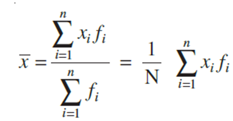
where    denotes the sum of the products of observations xi with their respective frequencies fi and  is the sum of the frequencies.

Then, we find the deviations of observations xi from the mean x and take their absolute values,

i.e.,| x- xi | for all i =1, 2,..., n.

After this, find the mean of the absolute values of the deviations, which is the required mean deviation about the mean. Thus

(ii) Mean deviation about median To find mean deviation about median, we find the median of the given discrete frequency distribution. For this the observations are arranged in ascending order. After this the cumulative frequencies are obtained. Then, we identify the observation whose cumulative frequency is equal to or just greater than N/2 , where N is the sum of frequencies. This value of the observation lies in the middle of the data, therefore, it is the required median. After finding median, we obtain the mean of the absolute values of the deviations from median .Thus,

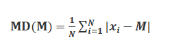
where  Median

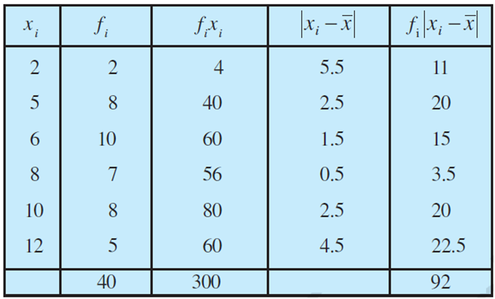
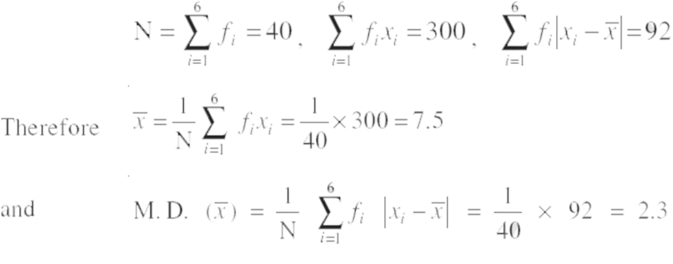
Example:  Find mean deviation about the mean for the following data :

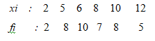
Solution:

Variance:

A variance of zero indicates that all the values are identical. It should be noted that variance is always non-negative- a small variance indicates that the data points tend to be very close to the mean and hence to each other while a high variance indicates that the data points are very spread out around the mean and from each other.

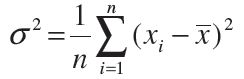
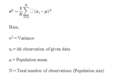
Mean of the squares of the deviations from mean is called the variance and is denoted by

s² (read as sigma square). Therefore, the variance of n observations x1, x2,..., xn is given by

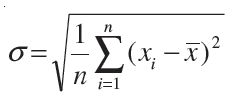
Standard Deviation :  In the calculation of variance, we find that the units of individual observations xi and the unit of their mean x are different from that of variance, since variance involves the sum of squares of (xi– x ). For this reason, the proper measure of dispersion about the mean of a set of observations is expressed as positive square-root of the variance and is called standard deviation. Therefore, the standard deviation, usually denoted by s

Properties of Variance

• It is always non-negative since each term in the variance sum is squared and therefore the result is either positive or zero.
• Variance always has squared units. For example, the variance of a set of weights estimated in kilograms will be given in kg squared. Since the population variance is squared, we cannot compare it directly with the mean or the data themselves.

Variance Formulas for UnGrouped Data

Variance Formulas for Grouped Data

Standard deviation of a discrete frequency distribution: Let the given discrete

frequency distribution be

 

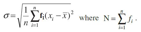
Standard deviation of a continuous frequency distribution: The given continuous frequency distribution can be represented as a discrete frequency distribution by replacing each class by its mid-point. Then, the standard deviation is calculated by the technique adopted in the case of a discrete frequency distribution.

If there is a frequency distribution of n classes each class defined by its mid-point

xi with frequency fi, the standard deviation will be obtained by

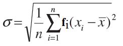
where  is the mean of the distribution and

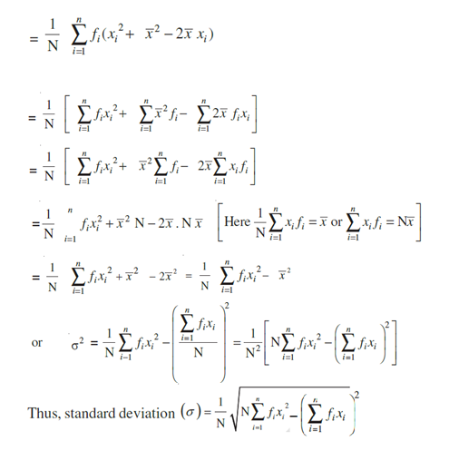
Another formula for standard deviation :

We know that

Variance (s2 )  =

Properties of Standard Deviation

• It describes the square root of the mean of the squares of all values in a data set and is also called the root-mean-square deviation.
• The smallest value of the standard deviation is 0 since it cannot be negative.
• When the data values of a group are similar, then the standard deviation will be very low or close to zero. But when the data values vary with each other, then the standard variation is high or far from zero.

Question: Find the variance for the following set of data representing trees heights in feet: 3, 21, 98, 203, 17, 9

Solution:

Step 1: Add up the numbers in your given data set.

3 + 21 + 98 + 203 + 17 + 9 = 351

Step 2: Square your answer:

351 × 351 = 123201

…and divide by the number of items. We have 6 items in our example so:

123201/6 = 20533.5

Step 3: Take your set of original numbers from Step 1, and square them individually this time:

3 × 3 + 21 × 21 + 98 × 98 + 203 × 203 + 17 × 17 + 9 × 9

Add the squares together:

9 + 441 + 9604 + 41209 + 289 + 81 = 51,633

Step 4: Subtract the amount in Step 2 from the amount in Step 3.

51633 – 20533.5 = 31,099.5

Set this number aside for a moment.

Step 5: Subtract 1 from the number of items in your data set. For our example:

6 – 1 = 5

Step 6: Divide the number in Step 4 by the number in Step 5. This gives you the variance:

31099.5/5 = 6219.9

Step 7: Take the square root of your answer from Step 6. This gives you the standard deviation:

σ =√6219.9 = 78.86634

The answer is 78.86.

Question :

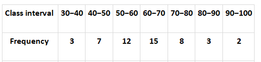
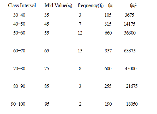
Calculate the variance for the following data:

Solution:

What Are the merits and demerits of range?

Merits

1. It is very easy to calculate and simple to understand.
2. No special knowledge is needed while calculating range.
3. It takes the least time for computation.
4. It provides a broad picture of the data at a glance.

Demerits

1. It is a crude measure because it is only based on two extreme values (highest and lowest).
2. It cannot be calculated in the case of open-ended series.
3. Range is significantly affected by fluctuations of sampling, i.e. it varies widely from sample to sample.

Merits and demerits of Quartile Deviation

Merits

1. It is also quite easy to calculate and simple to understand.
2. It can be used even in case of open-end distribution.
3. It is less affected by extreme values so, it a superior to ‘Range’.
4. It is more useful when the dispersion of the middle 50% is to be computed.

Demerits

1. It is not based on all the observations.
2. It is not capable of further algebraic treatment or statistical analysis.
3. It is affected considerably by fluctuations of sampling.
4. It is not regarded as a very reliable measure of dispersion because it ignores 50% observations.

What Are the merits and demerits of mean deviation?

Merits

1. It is based on all the observations of the series and not only on the limits like Range and QD.
2. It is simple to calculate and easy to understand.
3. It is not much affected by extreme values.
4. For calculating mean deviation, deviations can be taken from any average.

Demerits

1. Ignoring + and – signs is bad from the mathematical viewpoint.
2. It is not capable of further mathematical treatment.
3. It is difficult to compute when the mean or median is in fraction.
4. It may not be possible to use this method in case of open ended series.

Sample spaces, events and types of events, Algebra of events:

The set of all possible outcomes of a random experiment is called the sample space associated with the experiment.

Sample space is denoted by the symbol S.

Each element of the sample space is called a sample point.

 In other words, each outcome of the random experiment is also called sample point.

Example : Two coins (a one rupee coin and a two rupee coin) are tossed once.

Find a sample space.

Solution:

Heads on both coins = (H,H) = HH

Head on first coin and Tail on the other = (H,T) = HT

Tail on first coin and Head on the other = (T,H) = TH

Tail on both coins = (T,T) = TT

Thus, the sample space is S = {HH, HT, TH, TT}

Example : Consider the experiment in which a coin is tossed repeatedly until a head comes up. Describe the sample space.

Solution:

In the experiment

head may come up on the first toss, or the 2nd toss, or the 3rd toss and so on till head is obtained.

Hence, the desired sample space is  S= {H, TH, TTH, TTTH, TTTTH,...}

Event:

Any subset E of a sample space S is called an event.

Types of events:

1. Impossible and Sure Events :

The empty set f and the sample space S describe events.

In fact f is called an impossible event and S, i.e., the whole sample space is called the sure event.

Example:

let us consider the experiment of rolling a die. The associated sample space is

S = {1, 2, 3, 4, 5, 6}

Let E be the event “ the number appears on the die is a multiple of 7”.

E={} = f is an impossible event.

Let event F “the number turns up is odd or even”.

F= {1, 2, 3, 4, 5, 6} = S

Thus, the event F = S is a sure event.

1. Simple Event : If an event E has only one sample point of a sample space, it is

called a simple (or elementary) event.

In a sample space containing n distinct elements, there are exactly n simple events.

For example in the experiment of tossing two coins, a sample space is

S={HH, HT, TH, TT}

There are four simple events corresponding to this sample space. These are

E1= {HH}, E2={HT}, E3= { TH} and E4={TT}.

2. Compound Event: If an event has more than one sample point, it is called a

Compound event.

For example, in the experiment of “tossing a coin thrice” the events

E: ‘Exactly one head appeared’

F: ‘Atleast one head appeared’

G: ‘Atmost one head appeared’ etc.

are all compound events. The subsets of S associated with these events are

E={HTT,THT,TTH}

F={HTT,THT, TTH, HHT, HTH, THH, HHH}

G= {TTT, THT, HTT, TTH}

Algebra of events:

1. Complementary Event
2. The Event ‘A or B’
3. The Event ‘A and B’
4. The Event ‘A but not B’

i)  Complementary Event: For every event A, there corresponds another event Acalled the complementary event to A. It is also called the event ‘not A’.

For example, take the experiment ‘of tossing three coins’. An associated sample

Space  is S = {HHH, HHT, HTH, THH, HTT, THT, TTH, TTT}

Let  A= {HTH, HHT, THH} be the event ‘only one tail appears’

Clearly for the outcome HTT, the event A has not occurred. But we may say that the event ‘not A’ has occurred. Thus, with every outcome which is not in A, we say that ‘not A’ occurs.

Thus the complementary event ‘not A’ to the event A is

A`= {HHH, HTT, THT, TTH, TTT}

or  A¢ = {w : w Î S and w ÏA} = S – A.

ii)  The Event “ A or B  “ : Recall that union of two sets A and B denoted by A È B contains all those elements which are either in A or in B or in both.

When the sets A and B are two events associated with a sample space,

Then ‘A È B’ is the event ‘either A or B or both’. This event ‘A È B’ is also called ‘A or B’.

Therefore Event ‘ A or B ’ = A È B  = {w : w Î A or w Î B}

iii)  The Event ‘ A and B ’ : We know that intersection of two sets A Ç B is the set of

those elements which are common to both A and B. i.e., which belong to both ‘A and B’.

If A and B are two events, then the set A Ç B denotes the event ‘A and B’.

Thus, A Ç B = {w : w Î A and w Î B}

For example, in the experiment of ‘throwing a die twice’

Let A be the event ‘score on the first throw is six’ and

 B is the event ‘sum of two scores is atleast 11’ then

A = {(6,1), (6,2), (6,3), (6,4), (6,5), (6,6)}, and B = {(5,6), (6,5), (6,6)}

So  A Ç B = {(6,5), (6,6)}

Note that the set A Ç B = {(6,5), (6,6)} may represent the event ‘the score on the first throw is six and the sum of the scores is atleast 11’.

iii)  The Event ‘A but not B’ : We know that A–B is the set of all those elements

which are in A but not in B. Therefore, the set A–B may denote the event ‘A but not B ’.We know that  A – B = A Ç B´

Example:  Consider the experiment of rolling a die. Let A be the event ‘getting a prime number’, B be the event ‘getting an odd number’. Write the sets representing the events

(i) Aor B (ii) A and B (iii) A but not B (iv) ‘not A’.

Solution:  Here S = {1, 2, 3, 4, 5, 6}, A = {2, 3, 5} and B = {1, 3, 5}

Obviously

(i) ‘A or B’ = A È B = {1, 2, 3, 5}

(ii) ‘A and B’ = A Ç B = {3,5}

(iii) ‘A but not B’ = A – B = {2}

(iv) ‘not A’ = A¢ = {1,4,6}

Mutually exclusive events:

Two events A and B are called mutually exclusive events if the occurrence of any one of them excludes the occurrence of the other event, i.e., if they can not occur simultaneously. In this case the sets A and B are disjoint.

Example:

In the experiment of rolling a die, a sample space is

S = {1, 2, 3, 4, 5, 6}. Consider events, A ‘an odd number appears’ and B ‘an even

number appears’

Clearly the event A excludes the event B and vice versa.

In other words, there is no outcome which ensures the occurrence of events A and B simultaneously.

Here A = {1, 3, 5} and B = {2, 4, 6}

Clearly A Ç B = f, i.e., A and B are disjoint sets.

So two events A and B are called mutually exclusive events.

Note: Simple events of a sample space are always mutually exclusive.

if E1, E2, ..., En are n events of a sample space S and ifE₁ È E₂ È E₃ È E₄ È...... È E_n = S

then E1, E2, ...., En are called exhaustive events.

In other words, events E1, E2, ..., En are said to be exhaustive if atleast one of them necessarily occurs whenever the experiment is performed.

Further, if Ei Ç Ej = f for i ¹ j i.e., events Ei and Ej are pairwise disjoint and

, then events E1, E2, ..., En are called mutually exclusive and exhaustive events.

Example :  A coin is tossed three times, consider the following events.

A: ‘No head appears’, B: ‘Exactly one head appears’ and C: ‘Atleast two heads

appear’.

Do they form a set of mutually exclusive and exhaustive events?

Solution: The sample space of the experiment is

S = {HHH, HHT, HTH, THH, HTT, THT, TTH, TTT}

and A = {TTT}, B = {HTT, THT, TTH}, C = {HHT, HTH, THH, HHH}

Now

A È B È C = {TTT, HTT, THT, TTH, HHT, HTH, THH, HHH} = S

Therefore, A, B and C are exhaustive events.

Also, A Ç B = f, A Ç C = f and B Ç C = f

Therefore, the events are pair-wise disjoint, i.e., they are mutually exclusive.

Hence, A, B and C form a set of mutually exclusive and exhaustive events.

Axiomatic Approach to probability:

Axiomatic probability is a unifying probability theory in Mathematics. The axiomatic approach to probability sets down a set of axioms that apply to all of the approaches of probability which includes frequentist probability and classical probability. These rules are generally based on Kolmogorov's Three Axioms.

Axiomatic approach is another way of describing probability of an event. In this approach some axioms or rules are depicted to assign probabilities.

Let S be the sample space of a random experiment.

The probability P is a real valued function whose domain is the power set of S and range is the interval [0,1] satisfying the following axioms

1. For any event E, P (E) ³ 0
2.  (ii) P (S) = 1
3. If E and F are mutually exclusive events, then P(E È F) = P(E) + P(F).

P (E È f) = P (E) + P (f)

 P(E) = P(E) + P (f)

i.e. P (f) = 0.

Let S be a sample space containing outcomes w₁, w₂, ..., w_n .

i.e., S = {w₁, w₂, ..., w_n}

It follows from the axiomatic definition of probability that

(i) 0 £ P (w_i) £ 1 for each w_i Î S

(ii) P (w₁) + P (w₂) + ... + P (w_n) = 1

(iii) For any event A, P(A) = å P(w_i ), w_i Î A.

Example: A coin tossing

S={H,T}

P(H)= ½  ,P(T) = ½

i.e., each number is neither less than zero nor greater than 1

and P(H) + P(T) = ½ + ½  = 1

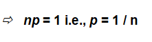
In fact, we can assign the numbers p and (1 – p) to both the outcomes such that

0 £ p £ 1 and P(H) + P(T) = p + (1 – p) = 1

This assignment, too, satisfies both conditions of the axiomatic approach of probability.

Hence, we can say that there are many ways (rather infinite) to assign probabilities to outcomes of an experiment.

Discrete and Continuous distributions:

A discrete distribution is one in which the data can only take on certain values, for example integers. 

Thus, in a discrete frequency distribution, the values of the variable are determined individually. The number of times each value occurs denotes the frequencies of the particular value or observation.

A continuous frequency distribution is a series in which the data are classified into different class intervals without gaps and their respective frequencies are assigned as per the class intervals and class width.

Continuous data is data that can take any value. Height, weight, temperature and length are all examples of continuous data.

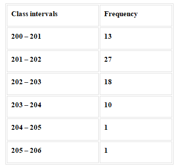
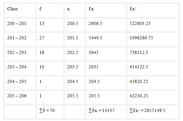
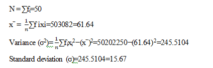
Question: Calculate the variance and standard deviation of the following continuous frequency distribution

Solution:

 

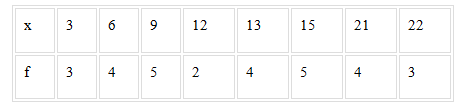
Example: Prepare a discrete frequency distribution table for the following data.

12, 21, 21, 3, 9, 3, 6, 12, 13, 21, 15, 22, 3, 6, 9, 9, 21, 22, 15, 13, 15, 9, 15, 6, 15, 13, 6, 9, 13, 22

Solution:

Given data:

12, 21, 21, 3, 9, 3, 6, 12, 13, 21, 15, 22, 3, 6, 9, 9, 21, 22, 15, 13, 15, 9, 15, 6, 15, 13, 6, 9, 13, 22

The discrete frequency distribution table is given as:

Frequency distributions analysis

Frequency distribution, in statistics, a graph or data set organized to show the frequency of occurrence of each possible outcome of a repeatable event observed many times. Simple examples are election returns and test scores listed by percentile. A frequency distribution can be graphed as a histogram or pie chart.

 Frequency is the number of times an event occurs. Frequency Analysis is an important area of statistics that deals with the number of occurrences (frequency) and analyzes measures of central tendency, dispersion, percentiles, etc.

 Whenever we want to compare the variability of two series with the same mean, measured in different units, we do not merely calculate the measures of dispersion. Still, we need such measures which are independent of the units. The measure of variability, independent of units, is called the coefficient of variation (CV). However, we know that the mean deviation and the standard deviation have the same units in which the data are given.

The coefficient of variation is defined as the percentage of standard deviation over mean. This can be calculated as:

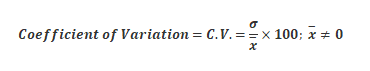
Here,  = Standard deviation of the data

 = Mean of the data

we calculate the coefficient of variance for each series. The series having greater C.V. is said to be more variable than the other. The series having lesser C.V. is said to be more consistent than the other.

Comparison of two frequency distributions with same mean:

Let x  and s₁ be the mean and standard deviation of the first distribution, and   and s₂ be the

mean and standard deviation of the second distribution.

It is clear from (1) and (2) that the two C.Vs. can be compared on the basis of values

of s1 and s2only.

Thus, we say that for two series with equal means, the series with greater standard

deviation (or variance) is called more variable or dispersed than the other. Also, the

series with lesser value of standard deviation (or variance) is said to be more consistent

than the other.

Question:

The below data shows the mean and variance of heights and the corresponding weights of the students of Class X:

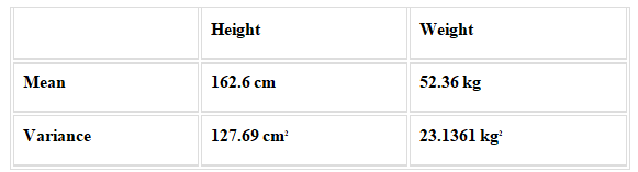
What can be said about the weights and the heights?

Solution:

For the given, we consider the heights of students as one series of data and weights as the other series of data.

So,

Mean of height = 162.6 cm

Variance of height = 127.69cm²

Therefore, standard deviation of height = √127.69 cm = 11.3 cm

Also,

Mean of weight = 52.36 kg

Variance of weight = 23.1361 kg²

Thus, the standard deviation of weight = √23.1361 kg = 4.81 kg

Now, we need to calculate the coefficient of variation for these two data sets to identify the relationship between them.

Using the coefficient of variation formula,

i.e. CV = (standard deviation/mean) × 100

For heights, the coefficient of variation (C.V.) = (11.3/162.6) × 100 = 6.95

For weights, the coefficient of variation (CV) = (4.81/52.36) × 100 = 9.18

Here, the C.V. of heights is lesser than the C.V. of weights.

Therefore, weights show more variability than heights.

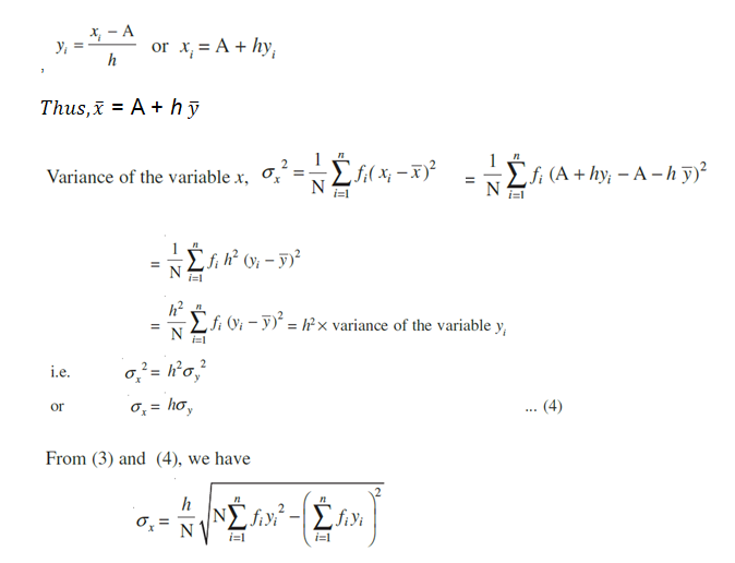
Shortcut method to find variance and standard deviation:

Shortcut method to find variance and standard deviation Sometimes the values of xi in a discrete distribution or the mid points xi of different classes in a continuous distribution are large and so the calculation of mean and variance becomes tedious and time consuming. By using step-deviation method, it is possible to simplify the procedure.

Let the assumed mean be ‘A’ and the scale be reduced to 1/h times (h being the width of class-intervals). Let the step-deviations or the new values be yi.

i.e 

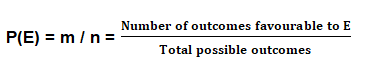
Probability of an event

The probability of an event is the proportion (relative frequency) of times that the event is expected to occur when an experiment is repeated a large number of times under identical conditions.

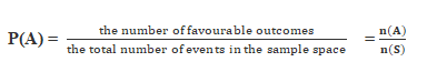
Where,

• P(A) is the probability of an event “A”
• n(A) is the number of favourable outcomes
• n(S) is the total number of events in the sample space

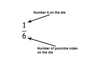
What is the probability to get a 6 when you roll a die?

A die has 6 sides, 1 side contain the number 6 that give us 1 wanted outcome in 6 possible outcomes.

Example:

Let us consider another experiment of ‘tossing a coin “twice”

The sample space of this experiment is S = {HH, HT, TH, TT}

P(HH) =1/4  , P(HT) = 1 / 7 , P(TH) = 2 / 7 ,  P(TT) = 9 / 28

The probability of the event E: ‘Both the tosses yield the same result’.

Here E = {HH, TT}

Now P(E) = S P(wi), for all wi Î E

= P(HH) + P(TT) = 1/4  + 9 / 28  = 4 /7

For the event F: ‘exactly two heads’, we have F = {HH}

P(F) = P(HH) = ¼

Probabilities of equally likely outcomes: Let a sample space of an experiment be

S = {w1, w2,..., wn}.

Let all the outcomes are equally likely to occur, i.e., the chance of occurrence of each

simple event must be same.

i.e. P(wi) = p, for all wi Î S where 0 £ p £ 1

Since  i.e., P(w1)+ P(w2)+ P(w3) + P(w4) + P(w5)+.....+ P(wn) = p + p + ... + p (n times) = 1

Let S be a sample space and E be an event, such that n(S) = n and n(E) = m. If each outcome is equally likely, then it follows that

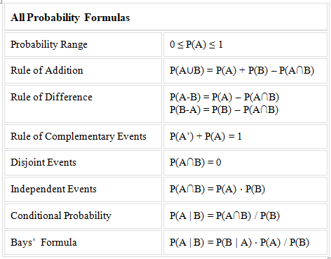
Basic Probability Formulas

Let A and B are two events. The probability formulas are listed below:

Probability of “not”, “and” and “or” events

If the events A and B are not mutually exclusive,

 the probability is: P(A or B) = P(A) + P(B) – P(A and B).

and

P(not A) = 1 – P(A)

Either/or probability refers to the probability that one event or the other will occur. For example, what is the probability that you will draw a Jack or a three from a normal deck of cards? Or, what is the probability that you will roll a 3 or a 5 when rolling a normal 6-sided die? To solve this type of probability problem, here is the formula you will use:

P(A or B) = P(A) + P(B)

To find the probability of each event, simply divide the amount of favorable events by the amount of total events. A favorable event is an event that you want to occur. In the earlier card question, the favorable event is drawing either a Jack or a three. The total number of events is the total number of things that could occur, whether favorable or not.

So, to continue on and solve this card drawing question, we have determined that A is the probability of drawing a Jack, and B is the probability of drawing a three.

There are 4 Jacks in a normal deck of cards, so the number of favorable events (drawing a Jack) is 4. The total number of events is 52 since there are 52 cards in a deck of cards. This means that the probability of drawing a Jack is 4/52, which can be reduced to 1/13.

P(B), or the probability of drawing a three, is also 1/13 because there are 4 threes in a deck of cards and, as before, there are 52 total cards in the deck.

To finish answering the question and find the probability of drawing either a Jack or a three, we use the equation P(A or B) = P(A) + P(B). P(A or B) is equal to 1/13 + 1/13, which is 2/13

To solve the dice question mentioned earlier, follow the same steps. P(A), or the probability of rolling a 3, is 1/6. There is one 3 (the favorable event) and 6 sides on the die (the total events).

P(B) is the probability of rolling a 5 and it's the same, 1/6. Therefore, the probability of rolling either a 3 or a 5 is P(A or B) is equal to 1/6 + 1/6, which is 2/6, or 1/3.

These events are called non-overlapping events, or events that are independent of each other. There are also overlapping events, which are events that are not independent of each other.

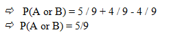
Example :  A die has sides numbered 1-9. You roll the die. What is the probability that the number you obtain is odd or prime.

Solution: Let A be the event that the number is odd and B the event that the number is a prime.

Then A and B are overlapping events 

since a number can be both prime and odd from among the numbers 1-9.

The odd numbers in 1-9 are 1, 3, 5, 7 and 9 (total of five), while the prime numbers in 1-9 are 1, 3, 5 and 7 (total of four). Hence the numbers in 1-9 that are odd AND prime are 1, 3, 5 and 7 (total of four).

Hence:

P(A or B) = P(A) + P(B) - P(A and B)

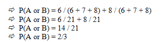
Example : A box has 6 red marbles, 7 blue marbles and 8 green marbles. You draw one marble at random from the box. What is the probability that the marble is red or green?

Solution:

Let A be the event that the marble is red and B be the event that the marble is green.

Since A and B are not overlapping, that marble cannot be both red AND green. So we get the probability as follows:

P(A or B) = P(A) + P(B)

Example : What is the probability that a card taken from a standard deck, is an Ace?

Solution:

Total number of cards a standard pack contains = 52

Number of Ace cards in a deck of cards = 4

So, the number of favourable outcomes = 4

Now, by looking at the formula,

Probability of selecting an ace from a deck is,

P(Ace) = (Number of favourable outcomes) / (Total number of favourable outcomes)

P(Ace) = 4/52

= 1/13

So we can say that the probability of getting an ace is 1/13.

Example : Calculate the probability of getting an odd number if a dice is rolled.

Solution:

Sample space (S) = {1, 2, 3, 4, 5, 6}

n(S) = 6

Let “E” be the event of getting an odd number, E = {1, 3, 5}

n(E) = 3

So, the Probability of getting an odd number is:

P(E) = (Number of outcomes favorable)/(Total number of outcomes)

= n(E)/n(S)

= 3/6

= ½

Example : Two students Anil and Ashima appeared in an examination. The probability that Anil will qualify the examination is 0.05 and that Ashima will qualify the examination is 0.10. The probability that both will qualify the examination is 0.02. Find the probability that

(a) Both Anil and Ashima will not qualify the examination.

(b) Atleast one of them will not qualify the examination and

(c) Only one of them will qualify the examination.

Solution: Let E and F denote the events that Anil and Ashima will qualify the examination,

respectively.

Given that P(E) = 0.05, P(F) = 0.10 and P(E Ç F) = 0.02.

Then

1. The event ‘both Anil and Ashima will not qualify the examination’ may be expressed as

E´ Ç F´.

Since, E´ is ‘not E’, i.e., Anil will not qualify the examination and F´ is ‘not F’,

i.e., Ashima will not qualify the examination.

Also E´ Ç F´ = (E È F)´ (by Demorgan's Law)

Now P(E È F) = P(E) + P(F) – P(E Ç F)

or P(E È F) = 0.05 + 0.10 – 0.02 = 0.13

Therefore P(E´ Ç F´) = P(E È F)´ = 1 – P(E È F) = 1 – 0.13 = 0.87

(b) P (atleast one of them will not qualify)

= 1 – P(both of them will qualify)

= 1 – 0.02 = 0.98

(c) The event only one of them will qualify the examination is same as the event either (Anil will qualify, and Ashima will not qualify) or (Anil will not qualify and Ashima will qualify)

i.e., E Ç F´  or  E´ Ç F,  where E Ç F´ and E´ Ç F are mutually exclusive.

Therefore, P(only one of them will qualify) = P(E Ç F´ or E´ Ç F)

=  P(E Ç F´) + P(E´ Ç F) = P (E) – P(E Ç F) + P(F) – P (E Ç F)

=  0.05 – 0.02 + 0.10 – 0.02 = 0.11

Example : If A, B, C are three events associated with a random experiment,

prove that

P(AÈBÈC) = P(A) + P(B) + P(C) - P(AÇB) - P(AÇC) – P ( B Ç C) + P ( A Ç B Ç C)

Solution: Consider E = B È C

so that

P (A È B È C ) = P (A È E )

= P(A) + P(E) - P(A ÇE) ............... (1)

Now

P(E) = P(BÈC) = P(B) + P(C) − P(BÇC) ... ……. (2)

Also AÇE = AÇ(BÈC) = (A ÇB)È(AÇC) [using distribution property of

intersection of sets over the union].

Thus

P(A ÇE) = P(A ÇB) + P(A ÇC)– P [(AÇB)Ç(AÇC)]

= P(AÇ B) + P(A ÇC) – P[A ÇBÇC] .................... (3)

Using (2) and (3) in (1), we get

P[AÈ BÈC] = P(A) + P(B) + P(C) - P(BÇC)– P(AÇ B) - P(A ÇC) + P(A ÇBÇC)