4. Frequency distributions analysis

Frequency distributions analysis

Frequency distribution, in statistics, a graph or data set organized to show the frequency of occurrence of each possible outcome of a repeatable event observed many times. Simple examples are election returns and test scores listed by percentile. A frequency distribution can be graphed as a histogram or pie chart.

 Frequency is the number of times an event occurs. Frequency Analysis is an important area of statistics that deals with the number of occurrences (frequency) and analyzes measures of central tendency, dispersion, percentiles, etc.

 Whenever we want to compare the variability of two series with the same mean, measured in different units, we do not merely calculate the measures of dispersion. Still, we need such measures which are independent of the units. The measure of variability, independent of units, is called the coefficient of variation (CV). However, we know that the mean deviation and the standard deviation have the same units in which the data are given.

The coefficient of variation is defined as the percentage of standard deviation over mean. This can be calculated as:

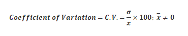
Here,  = Standard deviation of the data

 = Mean of the data

we calculate the coefficient of variance for each series. The series having greater C.V. is said to be more variable than the other. The series having lesser C.V. is said to be more consistent than the other.

Comparison of two frequency distributions with same mean:

Let x  and s₁ be the mean and standard deviation of the first distribution, and   and s₂ be the

mean and standard deviation of the second distribution.

It is clear from (1) and (2) that the two C.Vs. can be compared on the basis of values

of s1 and s2only.

Thus, we say that for two series with equal means, the series with greater standard

deviation (or variance) is called more variable or dispersed than the other. Also, the

series with lesser value of standard deviation (or variance) is said to be more consistent

than the other.

Question:

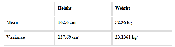
The below data shows the mean and variance of heights and the corresponding weights of the students of Class X:

What can be said about the weights and the heights?

Solution:

For the given, we consider the heights of students as one series of data and weights as the other series of data.

So,

Mean of height = 162.6 cm

Variance of height = 127.69cm²

Therefore, standard deviation of height = √127.69 cm = 11.3 cm

Also,

Mean of weight = 52.36 kg

Variance of weight = 23.1361 kg²

Thus, the standard deviation of weight = √23.1361 kg = 4.81 kg

Now, we need to calculate the coefficient of variation for these two data sets to identify the relationship between them.

Using the coefficient of variation formula,

i.e. CV = (standard deviation/mean) × 100

For heights, the coefficient of variation (C.V.) = (11.3/162.6) × 100 = 6.95

For weights, the coefficient of variation (CV) = (4.81/52.36) × 100 = 9.18

Here, the C.V. of heights is lesser than the C.V. of weights.

Therefore, weights show more variability than heights.