Unit 7 Statistics & Probability

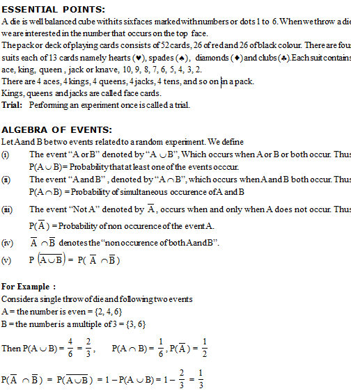
Introduction :
The chances of happening or non happening of an event when expressed quantitatively is called probability. There  are mainly two definitions of probability. 
(i) Experimental                                        (ii) Theoretical
In this chapter, we will study about these two types of probability. Experimental probability approach is when we toss the coin one – million times or 10 million times, we observe that as the number of tosses increases the experimental probability of a head or a tail comes close to 0.5. This is experimental approach to probability. The basic difference between the experimental and theoretical approach to probability is that former is based on what has actually happened but later is based on prediction of what will happen

Probability – A Theoretical Approach

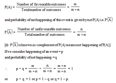
If an event A occurs m times and does not occurs n times. Then, the probability of occurence of event A, denoted by P(A) is given by 

Sum of the Probabilities of All the Elementary Event of an Experiment
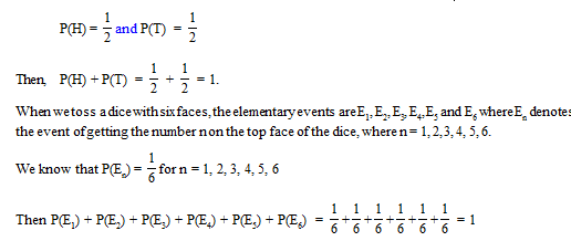
 If E₁ , E₂ ..........., En be the n elementary events associated with a random experiment having exactly n outcomes, then P(E₁) + P(E₂) + .......... + P(En) = 1. 
 For example, when we toss a coin, the resulting elementary events are H and T. 

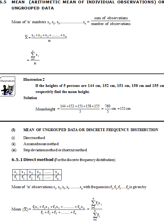
6.12     GRAPHICAL REPRESENTATION : 
    Graphical Representation : Many types of graphs are employed in statistics, depending upon the nauture of the data involved. Among these are
    (i)     Bar chart (or Bar graph)        
    (ii)     Histograms
    (iii)     Frequency Polygon        
    (iv)     Cumulative Frequency Curve (Ogive)
    (v)     Pie chart (or Pie graph or Pie Diagrams)

    Cumulative frequency Curve (Ogive) : 
    The term ‘ogive’ is pronounced as ‘ojeev’ and is derived from the word ogee. An ogee is a shape consisting of a concave arc flowing into a convex arc, so forming an S-shaped curve with vertical ends.

    Note :     For drawing ogives, it should be ensured that the class intervals are continuous. An ogive is the graphical representation of cumulative frequency distribution. We can construct two types of ogives. The first form is “less than ogive” and the second is “more than ogive”.
    In the “less than” method we start with the upper limit of the classes and go on adding the frequencies. When these are plotted, we get a rising curve.
    In the “more than” method we start with the lower limit of the classes and from the total frequencies we subtract the frequency of each class. When these are plotted, we get declining curve, e.g.

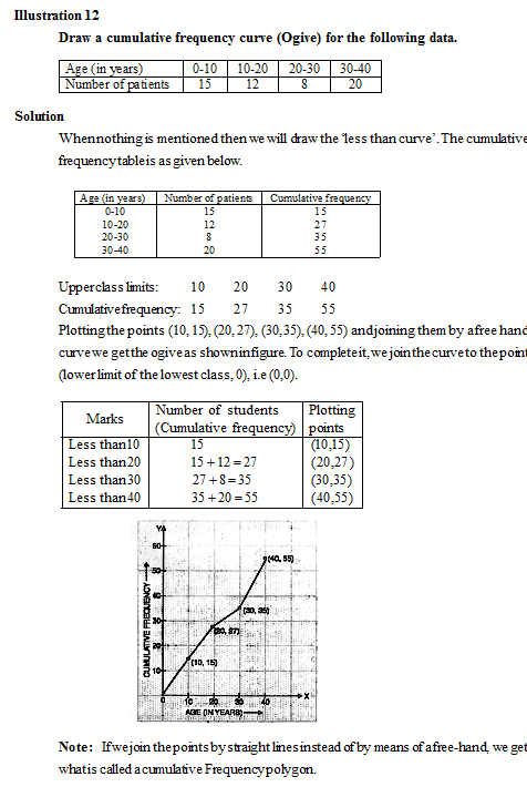
    6.12.1 The less than method  
    In this method the Ogive is cumulated upward. Scale the cumulative frequencies along the y-axis, and exact upper limits along the x-axis. The scale along the y-axis should be such as may accommodate the total frequency.
    Procedure:
    Step–1: Form the cumulative frequency table.
    Step–2: Mark the actual upper class limits along the x-axis.
    Step–3: Mark the cumulative frequencies of respective classes along the y-axis.
    Step–4: Plot the points (upper limits, corresponding cumulative frequency).
    To complete the ogive we also plot the point (lower limit of the lowest class, 0).
    Step–5: Join these points by a smooth curve.
    The curve so obtained is the required ogive.

Illustration : 1
            A box contains 3 blue, 2 white and 4 red marbles. If a marble is drawn at random from the box, what is the probability that it will be 
            (i) white ?                  (ii) blue ?            (iii) Red ?

Solution :
            Saying that a marble is drawn at random is a short way of saying that all the marbles are equally likely to be drawn. 
            Therefore, the number of possible outcomes = 3 + 2 + 4 = 9
            Let W denote the event ‘the marble is white’ , B denotes the event ‘the marble is blue’ and R denote the event ‘marble is red’.

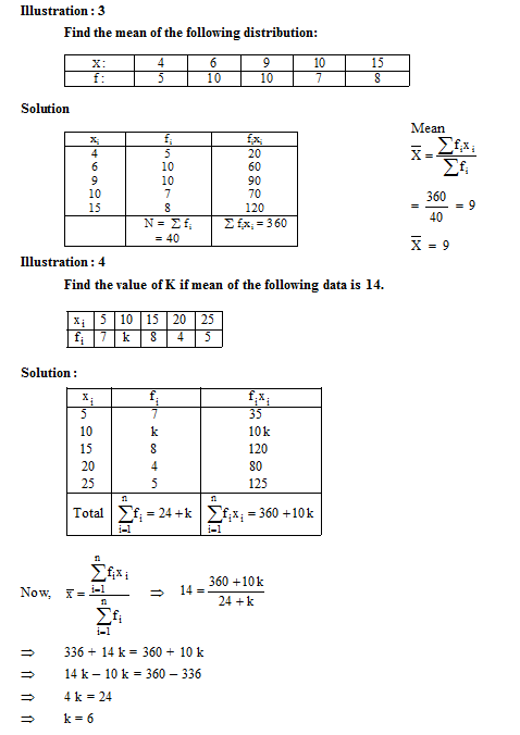
Illustration : 2
       Two coins are tossed simultaneously. Find the probability of getting 
       (i) two heads        (ii) at least one head        (iii) no head. 
 Solution : 
       Let H denotes head and T denotes tail. 
       On tossing two coins simultaneously, all possible outcomes HH, HT, TH, TT = 4.

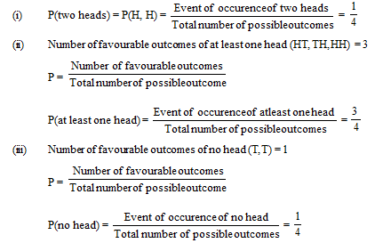
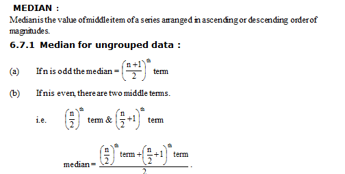
Illustration : 3
17 cards numbered 1, 2, 3, ........, 17 are put in a box and mixed throughly. One person draws a card from the box. Find the probability that the number on the card is 
 (i) odd        (ii) a prime    (iii) divisible by 3    (iv) divisible by 3 and 2 both. 
Solution :     
  (i) There are 9 odd numbered cards, namely 1, 3, 5, 7, 9, 11, 13, 15, 17. Out of these 9 cards one card can be drawn in 9 ways. 
      Favourable number of elementary events = 9
      Total number of elementary events = 17. 

(ii)     There are 7 prime numbered cards, namely. 2, 3, 5, 7, 11, 13, 17. Out of these 7 cards one card can be chosen in 7 ways.
         Favourable number of elementary events = 7 
         Total number of elementary events = 17

.

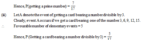
(iv)     If a number is divisible by both 3 and 2, then it is a multiple of 6. In cards bearing  number 1, 2, 3, ........17 there are only 2 cards which bear a number divisible by 3 and 2  both i.e., by 6.  These cards bear numbers 6 and 12. 
          Favourable number of elementary events = 2