 ACERISE INDIA
Median of Grouped Data Using Cumulative Frequency Table
Let us consider a group of numbers such as 17, 12, 15, 20, and 14. We can easily find the median of the given numbers. To find the median, first of all, we arrange the terms in increasing order. Then, we will have the sequence as 12, 14, 15, 17, and 20.
Here, we have 5 observations and the middle term is the 3rd term i.e., 15.
We know that median is the middle most observation of the data. Therefore, we can say 15 is the median of the given group of numbers.
However, we face problems when the data is given in grouped form. In such cases, we cannot use the above method to find the median. The method to find the median in such cases is different from the above. Let us discuss the method by taking an example.
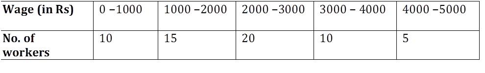
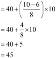
The following table shows the wages of 60 workers of a company. Let us find the median of wages of workers using this information.
Sometimes, the data is given as ‘less than type’ or ‘more than type’. In these cases, firstly we have to make cumulative frequency distribution table and then we can find the median using the same formula as in the previous example.
Let us discuss each of them briefly.
1. Less than Type
Let us consider the following table which contains the marks obtained out of 100 marks in an exam by the students of Grade 10 of a school.

To find the median of such data, first of all, we need to write the table in the form of class intervals and find the frequency of each class interval. The frequencies given for less than type table are cumulative frequencies. Now, the number of students obtaining marks in the class interval 0 − 10 is same as the number of students obtaining marks less than 10.
Therefore, the frequency of class interval 0 − 10 is 2. Now, the students obtaining marks less than 20 include the students of class interval 0 − 10 and 10 − 20. Therefore, frequency of class interval 10 − 20 = 6 − 2 = 4
Similarly, frequency of class interval 20 − 30 = 9 − 6 = 3
In this way, we can find the frequency of a class interval by taking the difference between the numbers of students of a group and its preceding group which is shown by the following table.

Since we have obtained the frequency distribution table, we can easily convert it into a cumulative frequency distribution table and follow the same method as we have studied in the beginning of this learning section. By doing so, we will easily find out the median of the given data.
2. More than Type
Let us consider the following table as the performance (in %) of taking calls by the customer care executives in a call centre.

To find the median of such data, first of all, we are required to write the table in the form of class intervals and find the frequency of each class interval. By looking at the given table, we write the class intervals of this data as 0 − 20, 20 − 40, 40 − 60, 60 − 80, and 80 − 100.
Now, the class more than 80 contains the customer care executives (C.C.E.) of class interval 80 − 100. Therefore, frequency of class interval 80 − 100 is 209. The class more than 60
contains the C.C.E. of class intervals 60 − 80 and 80 − 100. Therefore, frequency of class interval 60 − 80 = 585 − 209 = 376
Similarly, frequency of class interval 40 − 60 = 964 − 585 = 379
In this way, we can find the frequency of a class interval by taking the difference between the number of C.C.E .of a class and its following class as shown below.

Since we have obtained the frequency distribution table, we can easily convert it into a cumulative frequency distribution table and follow the same method as we have studied in the beginning. By doing so, we will easily find out the median of the given data.
Remember
• When a question is of more than or less than type, the cumulative frequency is always given.
• When the question is of more than type, the cumulative frequency is always in decreasing order.
• When the question is of less than type, the cumulative frequency is always in increasing order.
Let us solve some examples based on finding the median of less than type and more than type observations.
Example 1: The following table shows the literacy rate (in %) of 20 cities. Find the median literacy rate.

Solution:
The given table is of less than type. Therefore, the number of cities given in the table represents the cumulative frequencies. The frequencies and the class intervals are shown in the following table.

Here, number of observations, n = 20
![]()
The cumulative frequency greater than and nearest to 10 is 14.
∴ 40 − 50 is the median class.
l (lower limit of median class) = 40
h (class size) = 10
n (number of observations) = 20
cf = (cumulative frequency of the class preceding the median class) = 6
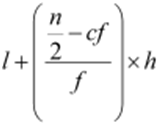
f (frequency of median class) = 8 Using the formula,
Median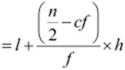
Therefore, 45% is the median literacy rate of 20 cities.
Example 2: If the median of the following distribution is 28.5, then find the value of x and y.

Solution:
First of all, we have to construct a cumulative frequency table.

It is given that n = 60
45 + x + y = 60
y = 15 − x … (1)
But, median = 28.5
i.e., median lies between the class interval 20 − 30.
Hence, median class = 20 − 30
Therefore, we have
l = 20, f = 20, cf = 5 + x, h = 10, and![]()
It is given that the median is 28.5.
 = 28.5
20 + ![]() = 28.5
= 28.5
20 + ![]() = 28.5
= 28.5
![]()
65 − x = 57
x = 65 − 57 = 8
Putting this value in equation (1), we obtain
y = 15 − x
y = 15 − 8 = 7
Hence, x = 8 and y = 7
Example 3: The following table shows the heights of buildings of a city. Find the median height.

Solution:
The given table is of more than type. Therefore, the number of buildings given in the table represents the cumulative frequencies. The frequencies and the class intervals have been shown in the following table.
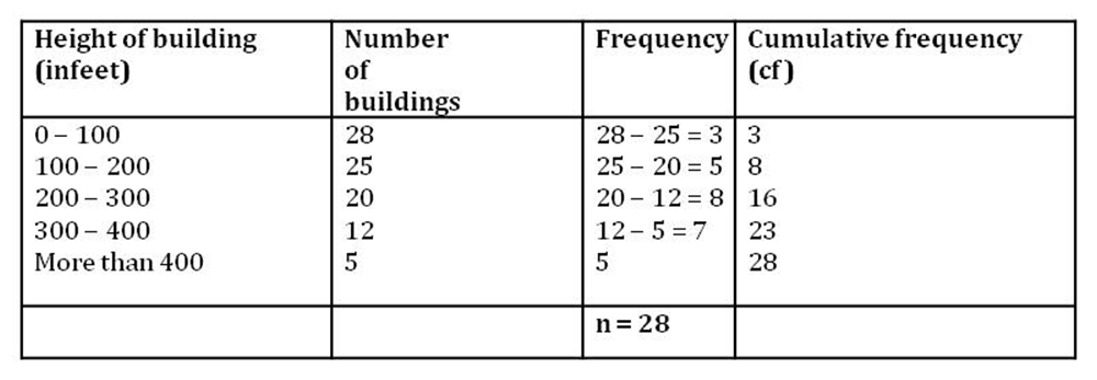
Here, n = 28
![]()
The cumulative frequency which is greater than and nearest to 14 is 16.
∴ 200 − 300 is median class.
We also have,
l (lower limit of median class) = 200
h (class size) = 100
n (number of observations) = 28
cf = (cumulative frequency of the class preceding the median class) = 8
f (frequency of median class) = 8 Using the formula, we have
Median
![]()
= 200 + 75
= 275
Hence,275 feet height is the median height.
Example 4: Lowest temperature of the day of a metro city was recorded for 30 consecutive days and the results are shown below:

Find the median lowest temperature.
Solution:
It can be observed that the class intervals in the given table are of inclusive type, so we need to convert them to exclusive type so that we can get continuous class intervals. Here, the difference between upper limit of a class and lower limit of next class is 0.1. On dividing this difference by 2, we get 0.05 which can be added to every upper limit and subtracted
from every lower limit to get new limits. These limits are known as class boundaries. Using these class boundaries, we can prepare cumulative frequency distribution table and thus, we can get continuous frequency distribution.
The new table can be prepared as follows:
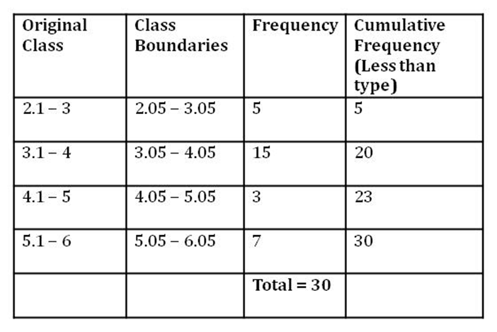
Here, n = 30
![]()
The cumulative frequency which is greater than and nearest to 15 is 20.
∴ 3.05 − 4.05 is median class. We also have,
l (lower limit of median class) = 3.05
h (class size) = 1
n (number of observations) = 30
cf = (cumulative frequency of the class preceding the median class) = 5
f (frequency of median class) = 15
Using the formula, we have
Median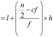
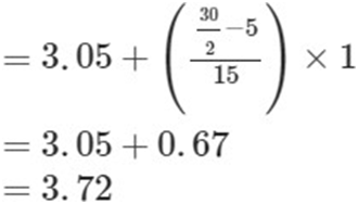
Hence, 3.72 °C is the median lowest temperature.
Median Of A Grouped Data By Constructing Ogive
A pictorial representation always gives a better understanding than a written statement. A graphical representation helps us in understanding of a given data in an easier and detailed manner. In order to understand the median of a grouped data properly, we have to draw an ogive.
Firstly, let us discuss what is an ogive?
“When the data is given as ‘less than’ or ‘more than’ type and a graph is plotted between either of the limits and the cumulative frequency, the smooth curve so obtained is known as ogive or cumulative frequency curve”.
Let us discuss with an example that how an ogive is helpful to find out the median of a grouped data.
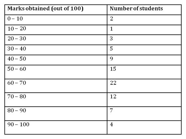
Let us consider that 80 students of a class appeared in a Geography test. The marks obtained (out of 100) by them are given in the following frequency distribution table.
Table - 1
We can write the above table in following two ways.
1. Less than type
2. More than type
1. For less than type
We can write the given table in less than type as follows.
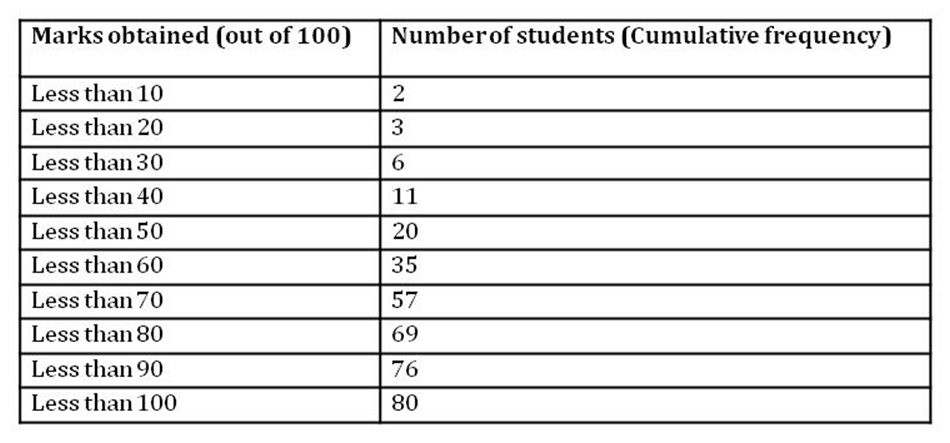
Construction of Ogive of less than type
The smooth curve drawn between the upper limits of class intervals and cumulative frequency is called cumulative frequency curve or ogive (of less than type). The upper limits of the intervals and cumulative frequency are shown in the above table.
The method of drawing an ogive of less than type is as follows.
1. Firstly we draw two perpendicular lines, one is horizontal (x-axis) and the other is vertical (y-axis), on a graph.
2. Now, we mark the upper limits on the horizontal line and the cumulative
frequencies on the vertical line by taking suitable scale.
(3) After this, we plot the points (10, 2), (20, 3), (30, 6), (40, 11), (50, 20), (60, 35), (70, 57),
(80, 69), (90, 76), (100, 80). These are the points corresponding to the upper limit and the cumulative frequency.
(4) Now, we join these points to obtain a smooth curve.
After following these steps, we obtain the following graph.
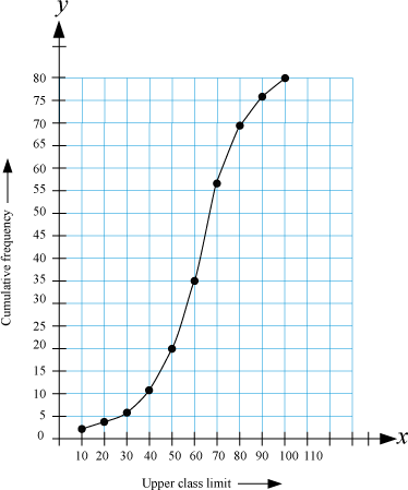
The smooth curve obtained in this figure is the ogive of less than type of the given data.
To find the median with the help of ogive
An important application of ogive in statistics is to find the median.
Let us see the method of finding the median through the same example. In the previous example, number of observations, n = 80

Mark the point 40 on the vertical line and then draw a horizontal line through this point. Let this horizontal line intersect the ogive at point A. Now, draw a vertical line through A. Median is the point at which this vertical line intersects the horizontal line.
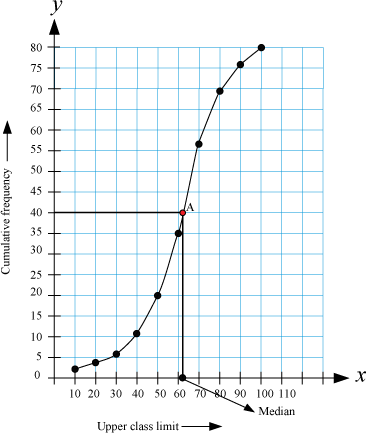
In this example, the median is 62 (approximately).
2. For more than type
We can write the given table for more than type as follows.
Marks obtained
Number of students (Cumulative frequency)
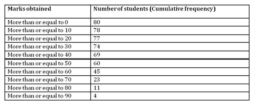
Construction of Ogive of more than type
The smooth curve drawn between the lower limits of class intervals and cumulative frequencies is called cumulative frequency curve or ogive (for more than type).
The method of construction of more than type ogive is same as the construction of less than type. For more than type ogive, we take the lower limits on x-axis and the cumulative frequencies on the y-axis. In the above table, the lower limits and the cumulative frequencies have been represented.
The ogive of more than type is obtained by plotting the points (0, 80), (10, 78), (20, 77),
(30, 74), (40, 69), (50, 60), (60, 45), (70, 23), (80, 11), (90, 4).
The ogive of more than type of the previous table has been shown below.
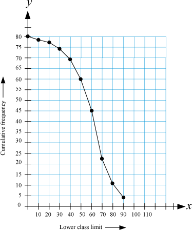
To find the median with the help of ogive
Number of observations, n = 80

Mark the point 40 on the vertical line and then draw a horizontal line from this point. Let this line intersect the ogive at point A. Now, draw a vertical line through A. Median is the point at which this vertical line intersects the horizontal line.
Hence, the median is 62(approximately).
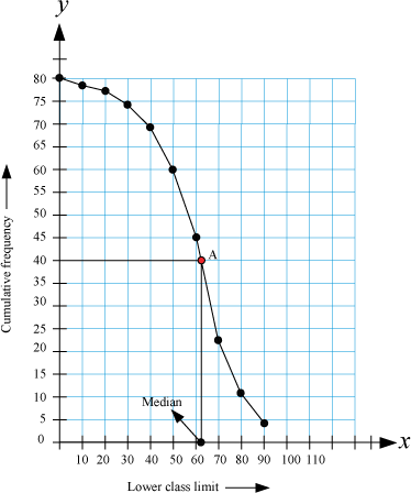
Relation between the ogive of less than type and more than type
Let us draw the graph of both less than type and more than type on the same graph paper.
We observe from the above graph that,
“If we construct a line parallel to y-axis through the point of intersection of both the ogives i.e., of less than type and more than type, then the point at which this line intersects x-axis represents the median of the given data”.
Let us solve some more examples to understand the concept better.
Example 1: The following distribution table gives the daily wages of 50 workers in a factory.
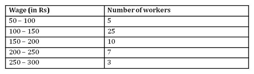
Convert it into a less than type distribution and draw its ogive. Solution:
We can write the given distribution table as a less than type distribution as follows.
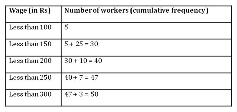
To obtain the ogive, we have to plot the points (100, 5), (150, 30), (200, 40), (250, 47), (300, 50) on a graph paper taking the upper limits on x-axis and the cumulative frequencies on y-axis.
The ogive obtained has been represented in the following figure.
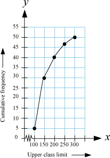
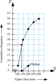
Here, n = 50
∴
First, we mark the point 25 on the vertical line and then draw a horizontal line through this point. Let this horizontal line intersect the ogive at point A. Now, draw a vertical line through point A. Median is the point where this vertical line intersects the x-axis. In this case, the value comes out to be 140. Hence, 140 is the median of the given distribution table.
Example 2: The following table shows the total monthly household expenditure of 100 families in a city.
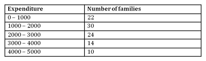
Convert it into a more than type of distribution and draw its ogive.
Solution:
We can write the given table in more than type as follows.
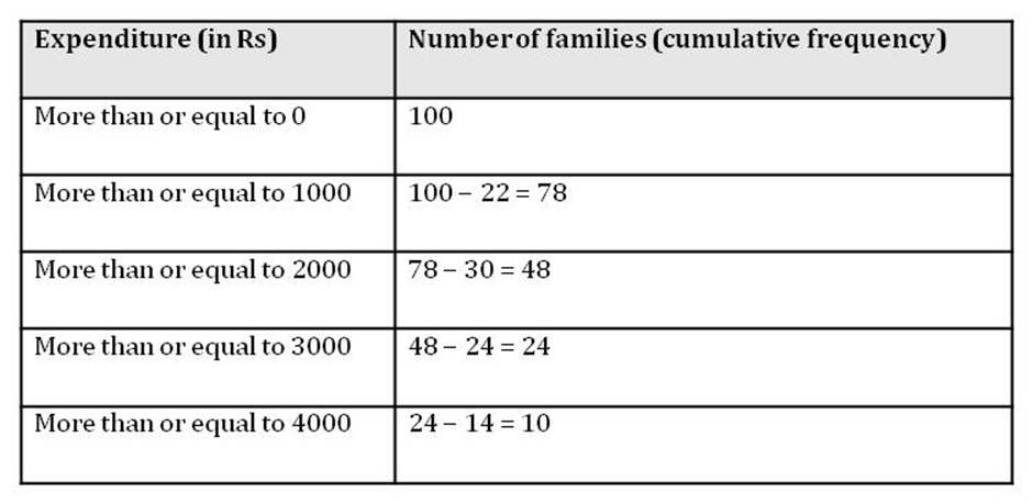
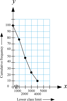
Now, we plot the points (0, 100), (1000, 78), (2000, 48), (3000, 24), (4000, 10) on a graph paper to obtain the ogive of more than type distribution.
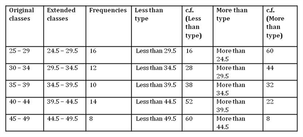
Example 3: The following table shows the rainfall (in mm) in 60 cities on a particular day.
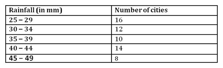
Draw both the ogives for this data on the same graph paper and find the median. Solution:
In the given table, the class intervals are of inclusive type, so we need to make them of exclusive type first. Now, a common table can be prepared for less than type and more than type cumulative frequencies to draw both the ogives on the same graph paper.
The table is given below.
Now, we plot the points (29.5, 16), (34.5, 28), (39.5, 38), (44.5, 52), (49.5, 60) on a graph paper to obtain the ogive of less than type distribution.
Also, we plot the points (24.5, 60), (29.5, 44), (34.5, 32), (39.5, 22), (44.5, 8) on the same graph paper to obtain the ogive of more than type distribution.
The graph is shown below:
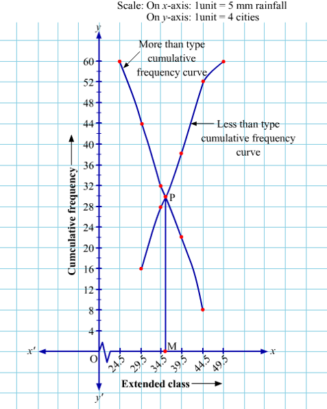
Point M represents the median which is approximately 36.
Relation Between Mean, Median, And Mode
We have studied three measures of central tendency - mean, median, and mode. But do you know that there is an empirical relationship between these three measures.
The relation between them is given by
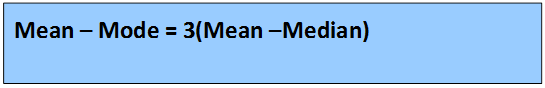
or
![]()
We can use this relationship to find the value of any of them, when the other two are known. It can also be used to check if the values of the three central tendencies obtained are correct or not as they will satisfy this relation. However, this relation is not always true.
First of all, let us verify it by taking an example.
Example: The following data shows the numbers of days for which the patients were hospitalized.
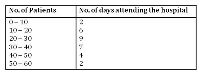
Justify the relationship between mean, median, and mode of the given data. Solution:
To verify the relation between mean, median, and mode, we have to find out their values from the given data and then substitute them to see the authenticity of the relationship.
Firstly, let us find the mean of the given data.
Mean
To find out the mean, we construct the following table.
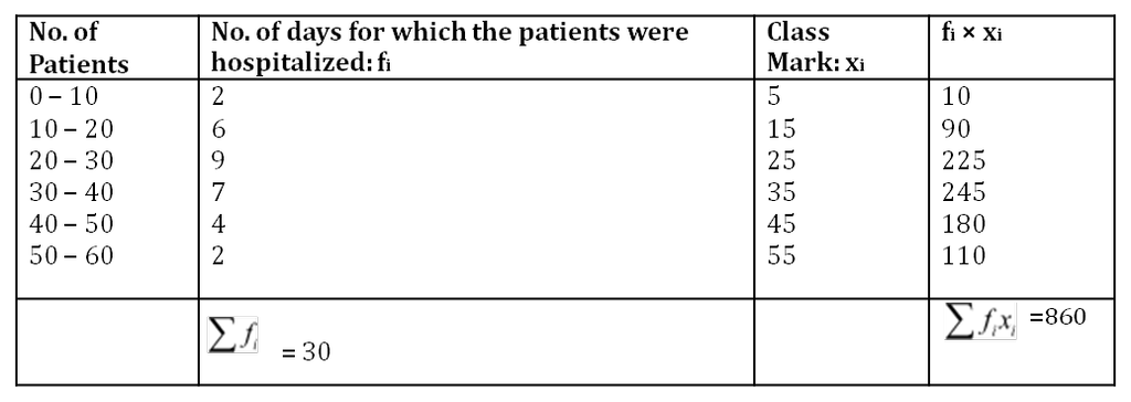
We know that, Mean =
=
Now, let us find the mode of the given set of data.
Mode
In the given table, 20 − 30 is the modal class as this group has the maximum frequency. From the table,
l = 20 (Lower limit of the modal class)
h = 10 (Class size)
f1 = 9 (Frequency of the modal class)
f0 = 6 (Frequency of the class preceding the modal class)
f2 = 7 (Frequency of the class succeeding the modal class)
Now, Mode =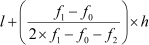
Mode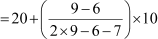
 Mode = 26
Median
To find out the median, we construct the following table.

Here, n = 30
 ∴
∴
The cumulative frequency greater than 15 is 17.
Hence, the median class is 20 − 30.
From the table,
l = 20 (Lower limit of median class)
cf = 8 (Cumulative frequency of class preceding the median class)
f = 9 (Frequency of median class)
h = 10 (Class size of the groups)
Now, Median
Median =
Median =
Now, Mode + 2 Mean = 26 + 2 ×
= 26 +
=
But, 3 Median = 3 × =
=  = Mode + 2 Mean
Hence it is verified that,
3 Median = Mode + 2 Mean
Let us go through few more examples to learn the application of the concept.
Example 1: For a certain frequency distribution, mean and median are obtained as 123.5 and 127 respectively. What is the value of mode?
Solution:
We have the relation
3 Median = Mode + 2 Mean
⇒ 3(127) = Mode + 2(123.5)
⇒ 381 = Mode + 247
⇒ Mode = 381 – 247
⇒ Mode = 134
Example 2: For a certain frequency distribution, median and mode are obtained as 55 and 70 respectively. What is the value of mean?
Solution:
We have the relation
3 Median = Mode + 2 Mean
⇒ 3(55) = 70 + 2 Mean
⇒ 165 = 70 + 2 Mean
⇒ 2 Mean = 165 – 70
⇒ 2 Mean = 95
⇒ Mean = 47.5
Example 3: For a certain frequency distribution, mean is 6 more than mode. Find the relation between median and mode.
Solution:
It is given that
Mean – Mode = 6 ...(1) We have the relation
Mean – Mode = 3(Mean – Median)
⇒ 6 = 3(Mean – Median)
⇒ Mean – Median = 2 ...(2)
On subtracting (2) from (1), we get Mean – Mode – (Mean – Median) = 6 – 2
⇒ Mean – Mode – Mean + Median = 4
⇒ Median – Mode = 4
Thus, median is 4 more than mode.